slama.dev

NNUEs, and Where to Find Them

Prokopakop · 7. 1. 2026 · 18 min read · Part 1, → Part 2 ← · [edit]

It turns out that it’s easier to start writing a chess engine than to stop writing it. This is something I wish I had known when I was starting, but it’s too late now so I might as well write another blog post to document the things that I’ve learned, and gloat a bit since the Prokopakop engine is now much stronger.

When I was initially writing the engine, I was eyeing the NNUE architecture, since replacing a painstakingly hand-crafted evaluation function with a gradient-(de)scented one sounded very appealing, but I wouldn’t spare it too much time since most of the engine was on fire.

Now, with the search functionality mostly in-place (modulo a few stragglers), the limiting factor is once again the evaluation, which is what I’ll spend most of this article on.

So, without further ado, let’s get some Elo and kop some prokops.

Search

Jokes aside, there are a few search techniques that I couldn’t cover in the previous blog post because it was getting too long, so I’ll sneak these in here and hope you won’t mind.

7cfbb74

PV-search

The Principal Variation search starts off, like most of the other optimizations that we discuss, with a simple observation – the principal line that we explored in the previous iteration of iterative deepening was hopefully good, so we assume that we won’t deviate from it in the next deepening iteration (except the last depth).

We can do this by doing two things:

• search the first move regularly, with a full window ([alpha, beta])
• for subsequent moves, search with a null window ([alpha, alpha + 1]), and re-search if it fails high

A null-window search only answers the question is this better than what I already have, which is exactly what we want in this case to confirm that the PV is the best. Since we’re usually right and null-window searches are much faster (only answers yes/no, not by how much better), this saves time, even though we sometimes have to re-search if we’re wrong about PV.

d00348d

History Heuristic

In the previous article, we have implemented many move ordering heuristics, such as MVV-LVA. While these were all useful in their own right, quiet moves have remained mostly untouched, since they’re… well… quiet, so it’s hard to judge whether one is better than another.

The only thing we’re doing right now for ordering quiet moves is the killer heuristic, which remembers moves that caused a beta cut-off in other branches in the same ply of the search tree. The history heuristic¹ is what you get when you take this to the extreme – if a move was good (i.e. caused a beta cut-off), we should prioritize it over other quiet moves in ALL future searched positions.

Implementation-wise, we can store [side][sq_from][sq_to], which will keep track of how good these moves were in the past, and will be updated as follows; if a move

• causes beta cutoff: [side][from][to] += depth * depth
• doesn’t improve alpha: [side][from][to] -= (depth * depth) / 2

The reason for using depth squared instead of constant values is that deeper cutoffs are more significant than shallower ones. To make sure entry values don’t explode, we can decay all entries over time (i.e. divide by 2 after each added move), or interpolate to some max value based on current value and depth (as Stockfish does).

7490eba

(Reverse) Futility Pruning

Futility pruning, as well as its Reverse Futility Pruning counterpart, prune positions that are futile (for either side), since they’re unlikely to change the outcome at that point.

What this means is that if we’re in a quiet position which, according to static evaluation, is hopeless and we are looking at a quiet move, it’s a reasonable assumption that it’s not going to help us and we can skip it, i.e. static eval + margin(depth) <= alpha. The higher depth we have remaining, the larger the margin should be for us to not miss tactics (i.e. [0, 100, 200, 300, ...]).

Similarly, if our position is amazing (static eval - reverse_margin(depth) >= beta), we can skip the branch entirely since, no matter the type of move, we will not get to play it anyway (again setting margins depending on the remaining depth).

85e2dae

Improving Time Management

I skipped this entirely in the previous post since I didn’t have time (heh, get it?), but since this commit makes significant improvements in how time per move is allotted, it’s a good idea to mention it here.

This is how much time Prokopakop currently assigns to each move:

1
2

let base_time = available_time / moves_until_increment.max(1);
let allocated_time = base_time + (increment * 8 / 10);

Since we’re usually playing games without a fixed move count until time control, moves_until_increment defaults to $30$ (or some other arbitrary value, based on how fast you want to decay), and so the remaining time decays exponentially as the moves go on.

While this sounds great on paper, implementing it like this is problematic – when the time runs out for a given step, the engine has to kill the current iterative deepening iteration and discard the result (unless you’re being very meticulous), since premature stopping can lead to incorrect move selection.

What this commit does to prevent this is to first calculate an estimate on how long the next iteration of iterative deepening will take, as a multiple of the previous (set to 2.5x). If the estimate exceeds the remaining time, the engine will skip the next iteration and return the current best result, since it’s likely that the time would be wasted as the iteration wouldn’t have completed.

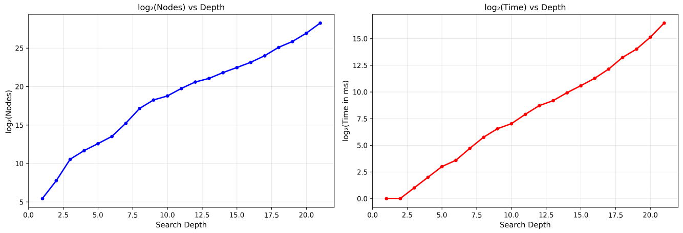
While crude, it matches the search quite well, as seen on a plot of time vs. depth when searching from the starting position. Although there are positions more/less complex than this, even a rough estimate is a good improvement over the naive kill+discard approach method.

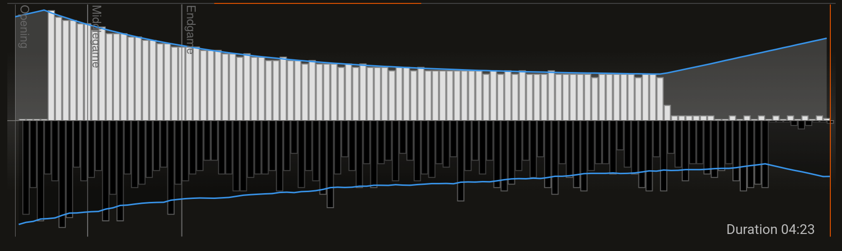
To see this in action, the image below shows the search time of an engine that doesn’t implement this (white), and an engine that does (black). Black won that game, because it’s my engine and I wouldn’t show you a loss.

c056f9b

Static Exchange Evaluation

During quiescence search, we’re resolving tactical sequences to get rid of the horizon effect. This usually involves captures, since these are at the heart of many tactics, so resolving them quickly is important.

Until now, we’ve resolved them by simply playing them out as recursive quiescence search calls, but we can do better. There are many capture sequences that we don’t ever need to consider, since they’re obviously bad (think Qxp followed by pxQ) and do not warrant a function call.

This is where static exchange evaluation comes in handy – instead of recursive calls, we will do the evaluation statically, calculating the overal result instead of recursing, since that’s the only thing we need in quiescence search.

While the implementation is a bit tricky to get both right and fast, the core idea is simple: there are pieces attacking a square with a piece. We want to calculate what is the material gain of the sequence by iteratively simulating the captures.

There are two observations that produce the algorithm that we’ll use. The first observation is that each of the players can stop capturing at any time. This means that while one player might have overwhelming material advantage (i.e. 2 queens), they shouldn’t capture a pawn if it’s being protected by a bishop.

The second observation is that it’s always optimal to capture with your lowest-value piece², since the opponent can always chose to stop capturing and so you didn’t help anything by sending higher-valued pieces earlier.

Here is the algorithm in a nutshell:

 1
 2
 3
 4
 5
 6
 7
 8
 9
10
11
12
13
14
15
16
17
18
19
20
21
22
23
24
25
26
27
28
29
30
31
32
33
34
35

let mut gains = [0.0f32; 16];  // max 16 captures
let mut depth = 1;

// Player 1 starts with the value of the piece they captured
let mut captured_value = get_see_piece_value(target_piece);

// Simulate exchange
loop {
    // Find smallest attacker for current side
    let (attacker, attacker_sq) = match self.get_smallest_attacker(square, side, occupied) {
        Some(sq) => sq,
        None => break,
    };

    // Store what we're capturing
    gains[depth] = captured_value;

    // Update for next iteration
    occupied &= !attacker_sq.to_mask();  // take piece
    captured_value = get_see_piece_value(attacker);
    side = !side;
    depth += 1;

    if depth >= 16 {
        break;
    }
}

// Minimax: each side chooses stop vs continue
while depth > 1 {
    depth -= 1;
    gains[depth] -= gains[depth + 1].max(0.0);
}

gains[1]

The core of the algorithm is in the final while loop – going from the end, each player makes the decision to stop capturing at that point if it’s not optimal for them (this is what max is doing). Since we’re doing this as negamax (always subtracting and thus swapping between the colors), the player will never want to play out a sequence that will yield a negative score, which is what we’re calculating by accumulating it from the end.

Besides quiescence search, you can use SEE to order capture moves – a lot of engines (mine included) do

since good captures tend to be better than the bad ones.

Evaluation

With the search functionality working reasonably well, we can focus on improving the evaluation.

The current way we’re doing it will not scale well, as it’s hand-crafted. We can improve it up to a point, but wouldn’t it be so much easier to descend some gradients instead?

a91a3f2~5063949

King Safety

Before we proceed to NNUEs, I’ve made some final improvements to the hand-crafted evaluation, namely king safety. Until now, I haven’t really paid attention to king safety, but it is arguably one of the most important parts of eval, as a king in danger can easily add $\pm 500$ centipawns.

The implementation penalizes a few things; namely:

• missing pawn shield in front of the king,
• (semi)-open files next to the king and, most importantly,
• attacks near the king (in the king zone), weighted by the attacker

The first two are pretty self-explanatory, but the third one is interesting. The idea behind it is that the more attacks there are around the king, the more exposed it is, with the values per attacked square being

1
2
3
4
5

const PAWN_ATTACK_WEIGHT: f32 = 1.0;
const KNIGHT_ATTACK_WEIGHT: f32 = 2.0;
const BISHOP_ATTACK_WEIGHT: f32 = 2.0;
const ROOK_ATTACK_WEIGHT: f32 = 3.0;
const QUEEN_ATTACK_WEIGHT: f32 = 5.0;

and the area around consisting of a $3 \times 4$ square like so:

8 ........
7 ..♗.....
6 ...\....
5 ....!••.  the bishop hits
4 ....•!•.  3 squares, adding
3 ....•♚!.  penalty of 3x2=6
2 ....•••\
1 ........
  abcdefgh

To further emphasise that king safety is important, the penalty increases quadratically since danger doesn’t increase linearly – the more attackers, the worse it gets, by a lot.

Removing Schizophrenia

I found this commit when looking through the Git history and thought it was funny.

1

* 3d536e8 | 2025-09-30 | xiaoxiae | make the engine not schizophrenic

I did not remember what I did, and as it’s not particularly descriptive, I wondered what it contained. Running git show revealed the following:

1
2

-    -danger * danger / SQUARE_ATTACK_FACTOR
+    -(danger * danger) * SQUARE_ATTACK_FACTOR

This, with SQUARE_ATTACK_FACTOR being 1/50 effectively meant that before this commit, the engine was extremely paranoid about king safety and would do anything to keep the king safe.

I stand by the commit message.

9cfd936~current

NNUEs

Ǝfficiently Updatable Иeural Иetworks are a relatively new addition to chess engines (~2018, ~2020 in Stockfish), and have revolutionized chess engines unlike (arguably) anything that came before them.

Traditionally, an evaluation function would be fast and hand-crafted (possibly tuned via a learning algorithm), due to the fact that a quicker evaluation function means deeper search and thus (generally) a better engine. This can work fine initially, but as the complexity of the function and the number of parameters increase, hand-crafting and tuning quickly becomes infeasible.

With the advent of AlphaZero, neural networks came into the chess engine scene in a big way, as AlphaZero decisively defeated Stockfish, the best chess engine in the world at the time. It used Monte-Carlo Tree Search instead of alpha-beta, since the evaluation was significantly slower than a standard evaluation function (around 1000x), and it wouldn’t get too far going layer-by-layer.

Although the AlphaZero architecture was markedly different from classical chess engines and so couldn’t be immediately applied, its massive success raised an important question – would a small, carefully designed neural network, outperform hand-crafted evaluations?

Spoiler alert: yes.

Overview

Let’s say we want to evaluate a chess position using a neural network. The simplest thing we could do is to use a fully-connected network (see my ML course lecture notes for more details) with a suitable input and a single scalar output, which would tell us how good the position is.

The input can take many shapes, but the easiest would be a one-hot encoding of the board state, with each combination of square/piece/color corresponding to a single neuron, for a total of

input neurons.

The core idea behind NNUEs is the following: after a move is made, what values do we actually need to change to update the network? It will of course be the neurons in the first layer corresponding to the changed pieces, but how about the others?

Since we’re dealing with a fully connected network, we only need to update the values of the neurons that the changed input neuron is connected to (and the subsequent layers), instead of having to re-calculate the entire network. If the network is shallow enough (i.e. 1 hidden layer), the number of operations needed for the evaluation then equals the size of the hidden layer!

Since the first hidden layer repeatedly adds/subtracts values based on how the pieces move on the board, it is referred to as the accumulator. Usually, two accumulators are used instead, one for the side to move and the other for the side not to move, since this takes full advantage of the game symmetry and allows the network to learn different features for both the “player” (positive) and “opponent” (negative).

Updating code for adding a piece to the board is then as simple as

 1
 2
 3
 4
 5
 6
 7
 8
 9
10
11
12
13
14
15
16
17
18
19
20

pub fn add_piece(square: Square, piece: Piece, color: Color, net: &Network) {
    // We're updating two accumulators, one from each point of view
    // 
    // In practice, we'll just call one 'white', the other 'black'
    // and swap them during evaluation, since the side-to-move switches
    let white_idx = Self::calculate_white_feature_idx(square, piece, color);
    let black_idx = Self::calculate_black_feature_idx(square, piece, color);
    
    self.white_accumulator.enable_index(white_idx, net);
    self.black_accumulator.enable_index(black_idx, net);
}

pub fn enable_index(&mut self, idx: usize, net: &Network) {
    let weights = &net.weights[idx].vals;
    
    // Accumulate weights for the activated neuron
    for (acc, weight) in self.vals.iter_mut().zip(weights) {
        *acc += weight;
    }
}

(analogously for removing a piece), and evaluate as

1
2
3
4
5
6
7
8
9

pub(crate) fn evaluate(&self) {
    let net = get_network();
    
    // Flip accumulators according to side-to-move
    match self.side == Color::White {
        true => net.evaluate(&self.white_accumulator, &self.black_accumulator),
        false => -net.evaluate(&self.black_accumulator, &self.white_accumulator),
    }
}

with the core net.evaluate function defined as:

 1
 2
 3
 4
 5
 6
 7
 8
 9
10
11
12
13
14
15
16
17
18
19
20
21
22
23
24
25
26
27

//
// https://github.com/jw1912/bullet/blob/main/examples/simple.rs
// 
impl Network {
    /// Calculates the output of the network, starting from the already
    /// calculated hidden layer (done efficiently during makemoves).
    pub fn evaluate(&self, us: &Accumulator, them: &Accumulator) -> f32 {
        // Initialise output.
        let mut output = 0.0;
    
        // Side-To-Move Accumulator
        for (&input, &weight) in us.vals.iter().zip(&self.output_weights[..HIDDEN_SIZE]) {
            output += screlu(input) * weight;
        }
    
        // Not-Side-To-Move Accumulator
        for (&input, &weight) in them.vals.iter().zip(&self.output_weights[HIDDEN_SIZE..]) {
            output += screlu(input) * weight;
        }
    
        // Add bias.
        output += self.output_bias;
    
        // Apply eval scale.
        output * SCALE
    }
}

Neat!

While this will work and you can train a really good chess engine this way, NNUEs have a few more tricks up their sleeve to make them faster and more accurate.

Quantization

Quantization has become a rather well-known term in these times of LLMs. By quantizing a network, we are converting the network layers to use integer types (i.e. f32 -> i16), since they have faster multiplication. This can be done by simply multiplying by a constant factor (say Q) and rounding to the nearest integer.

This will mean that we have to keep track of the current quantization factor so we can de-quantize as we go through the layers, and that the more layers the network has, the more the quantization errors propagate though the network. Luckily, these are non-issues since our network is very shallow – it’s not difficult to track it and the errors will be negligible.

While the details are heavily dependent on the network architecture, I’ll walk through how the one in Prokopakop works. I’m using the Bullet library for training NNUEs (Rust), although you could just as well use Pytorch (Python) or some other ML library. We’ll be quantizing the input layer to QA and the hidden layer to QB, and will use SCReLU as the activation function, yielding the following network architecture:

   side        side
    to        not to
   move        move
   acc.        acc.
    │           │
    ↓           ↓
   Linear(768, 128)      // quant = QA
    │           │
    ↓           ↓
 SCReLU()    SCReLU()    // quant = QA * QA
    │           │
    │  Concat   │
    └─────┬─────┘
          │
          ↓
    Linear(256, 1)       // quant = QA * QA * QB
          │
          ↓
       Output

You might think that it’s strange for the quantization to have an extra QA, but that comes from the fact that we’re using SCReLU, which squares the input.

Putting this together, we get

 1
 2
 3
 4
 5
 6
 7
 8
 9
10
11
12
13
14
15
16
17
18
19
20
21
22
23
24
25
26
27
28
29
30
31
32
33
34
35
36

//
// https://github.com/jw1912/bullet/blob/main/examples/simple.rs
// 
impl Network {
    /// Calculates the output of the network, starting from the already
    /// calculated hidden layer (done efficiently during makemoves).
    pub fn evaluate(&self, us: &Accumulator, them: &Accumulator) -> i32 {
        // Initialise output.
        let mut output = 0;

        // Side-To-Move Accumulator
        for (&input, &weight) in us.vals.iter().zip(&self.output_weights[..HIDDEN_SIZE]) {
            output += screlu(input) * i32::from(weight);
        }

        // Not-Side-To-Move Accumulator
        for (&input, &weight) in them.vals.iter().zip(&self.output_weights[HIDDEN_SIZE..]) {
            output += screlu(input) * i32::from(weight);
        }

        // Reduce quantization from QA * QA * QB to QA * QB,
        // since bias has been quantized with QA * QB only.
        output /= i32::from(QA);

        // Add bias.
        output += i32::from(self.output_bias);

        // Apply eval scale.
        output *= SCALE;

        // Remove quantisation altogether.
        output /= i32::from(QA) * i32::from(QB);

        output
    }
}

Output Buckets

I feel like I say this all the time in the chess articles that I write, but the core idea behind this is rather simple. The evaluation priorities based on the current phase of the game change drastically, which was reflected in our previous hand-crafted evaluation function in a number of ways, such as the changing piece table values.

Output Buckets are just a fancy way of doing this for NNUEs, where we have multiple output weights/biases and pick one based on the current phase of the game (determined by remaining material). Prokopakop uses 8, but any reasonable number will do – increasing will give you more granular weights for different stages of the game, but also increase the size of the network which may not be desirable since it will be harder to train.

There are similar more advanced techniques that can do this for input such as king input buckets and, to some extent, horizontal mirroring, but these usually only pay off, as I’ve mentioned, if you have massive amounts of training data.

Speaking of which…

Gathering data

To gather training data, I made the bot play with itself self-play, using a fixed depth of 8-12 and randomizing the first 1-6 moves, generating approximately 500 positions / second for approximately 11.5 days, amounting to approximately 500 million positions (about 32% unique).

This was not done at the same time, but in a bootstrapped manner:

1. self-play + evaluate to obtain training data (~100m positions at a time),
2. train NNUEs with different hyperparameters (LR, gamma),
3. run a tournament to compare, picking the best one and
4. repeat (1) for as many iterations as you’d like.

While the parameters will heavily depend on your particular network architecture and evaluation function, deduplicating positions was critical for my NNUEs to perform as they would otherwise overfit and lead to unstable results.

Results

Looking at the Elo progression below, it is safe to say that NNUEs helped, achieving a +200 elo increase over the non-NNUE version, which is almost the same as the increase of all of the search techniques combined (as the first functional state the engine was in was around ~1800).

I am not sure if this is because the engine still sucks or because NNUEs are just that good; either way I am not complaining and will continue training my silly little networks until the day I die.

Resources

• Chess Programming Wiki – an extremely well-written wiki that I took the vast majority of algorithms and techniques from.
• Bullet and its examples – a ML library for training NNUEs.