slama.dev

Generative Neural Networks

notes · 18. 10. 2023 · [edit]

• Introduction to generative modeling
• Warm up: 1D generative models
  • Classical approaches
• Warmed up: more dimensions!
  • Extensions of classical approaches
  • What if $p(X)$ must be learned?
  • Reducing $p(X)$ to many 1-D distributions
• Measuring model quality
  • Forward KL divergence
  • Reverse KL divergence
  • Comparison (forward x reverse)
  • Maximum Mean Discrepancy
• Generative Modeling with NN
  • Autoencoder
  • Generating data
• Generative Adversarial Networks (GANs)
• Normalized Flows (NF)
  • (2) Calculating $\det \mathcal{J}_f$
  • (1) Ensuring that $f(X)$ is invertible and computable
  • Summary
  • RealNVP
  • Spline coupling
  • Conditional derivatives
• Simulation-based inference (SBI)
  • Main tasks of SBI
  • Classical approaches for inverse inference
  • Doing it better with NN
  • Validation of generative models (especially SBI)
  • Validation of SBI
• Epidemology: SIR model
  • Making things more complex (because we can)
  • Checking if the simulation is realistic
  • Hierarchical models for SBI
• SINDy-Autoencoders
• Physics-informed Neural Networks (PINNs)
• State-of-the-art generative modeling
• Free-form flows
• Injective flows
• Bottleneck Free-form Flows

Note: these notes are in a pretty questionable state (at least after the first few lectures) – there are lot of TODOs that I won’t do. If you’re taking this class and have better notes, I’d be happy to update the website.

Preface

This website contains my lecture notes from a lecture by Ullrich Köthe from the academic year 2023/2024 (University of Heidelberg). If you find something incorrect/unclear, or would like to contribute, feel free to submit a pull request (or let me know via email).

Introduction to generative modeling

• assumption:
  • “nature” works according to some hidden mechanisms (complicated probability distribution)
  • $X$ is sampled from the true probability / generating process $X \sim p^*(X)$ (or $\hat{p}$)
  • we have a training set $TS = \left\{X_i \sim p^{*}(X)\right\}_{i=1}^n$
    • use $TS$ to learn $p(X) \approx p^*(X)$
• goal:
  • find approximation $X \sim p(X)$ (for $\hat p$)
• two aspects of generative modeling (neural network can usually do both):
  1. inference – given some data instance $X_i$, calculate value of $p(X_i)$
  2. generation – create synthetic data $X \sim p(X)$ which is indistinguishable from real data $X \sim p^{*}(X)$
• downstream benefits of generative modelling
  • powerful tool for humans (e.g. chat bot as personal teacher)
    • great for things that are well-established
    • poor for things that aren’t (tends to hallucinate)
  • helps to produce insight: identify important factors influencing the outcome
    • ex. “symbolic regression”: find / learn analytic formulas to explain the reality (vanilla neural networks are black boxes)
  • use $p(X)$ for decision making: is treatment $A$ better than treatment $B$ for patient $X$?

What I cannot create, I do not understand. (Richard Feynman)

Warm up: 1D generative models

Basic principle: $p(X)$ is complicated $\implies$ reduce it to something simple.

• introduce new variable (“code”) $Z = f(X)$ for $f$ deterministic function s.t. the $q(Z)$ distribution is simple
  • we’ll be actually doing it he other way – pick $q(Z)$ and learn $f$ (will be a NN)
• for generative modeling to work, we additionally require that $f(X)$ is invertible
  • if $X \sim p(X) \implies Z = f(X) \sim q(Z)$ – inference direction
  • if $Z \sim q(Z) \implies X = f^{-1} \sim p(X)$ – generative direction
    • called “inverse transform sampling’
• consequence in 1-D is that $f(X)$ must be a monotonic function (increasing by convention)
  • $\forall x\ \frac{d}{dx}f(x) \ge 0$ (strictly monotonic requires $> 0$)
• universal property of monotonic functions (saw proof in the lecture): $$\frac{d}{dx} f(X) \mid_{x=x_0} = \frac{1}{\frac{d}{dz} f^{-1}(Z) \mid_{z=f(x_0)}}$$

Apply to probability distribution:

• define mass in interval $x_0, x_1$ as $m(x_0, x_1) = \int_{x_0}^{x_1}p(x)\;dx$
• for the Gaussian distribution, $m(-\sigma, \sigma)$ gives about $0.68$ ($-2\sigma$ gives $0.95$)
• $f(x)$ is permissible, if for every interval $(x_0, x_1)$: $$\int_{x_0}^{x_1}p(x)\;dx=\int_{f(x_0)}^{f(x_1)}q(z)\;dz$$

Now we can substitute $z = f(z), dz = f'(x) dx, x_0 = f^{-1}(z_0), x_1 = f^{-1}(z_1)$, getting $$\int_{f^{-1}(f(x_0))}^{f^{-1}(f(x_1))} q(z=f(x)) f'(x)\;dx$$ which must hold for any interval $x_0, x_1$, meaning $$\boxed{p(x) = q(z=f(x)) f'(x)}$$ which is called the change-of-variables formula, allowing us to express the complex distribution in terms of the simple distribution, transformation and its derivative (this is where the fact that it’s always positive comes in handy, since it’s just a scaling factor).

For 1D, $q(Z) \sim \text{uniform}(0, 1)$ works well (numerically easy, a generator is available anywhere)

• e.g. Mersenne twister (based on Mersenne primes)
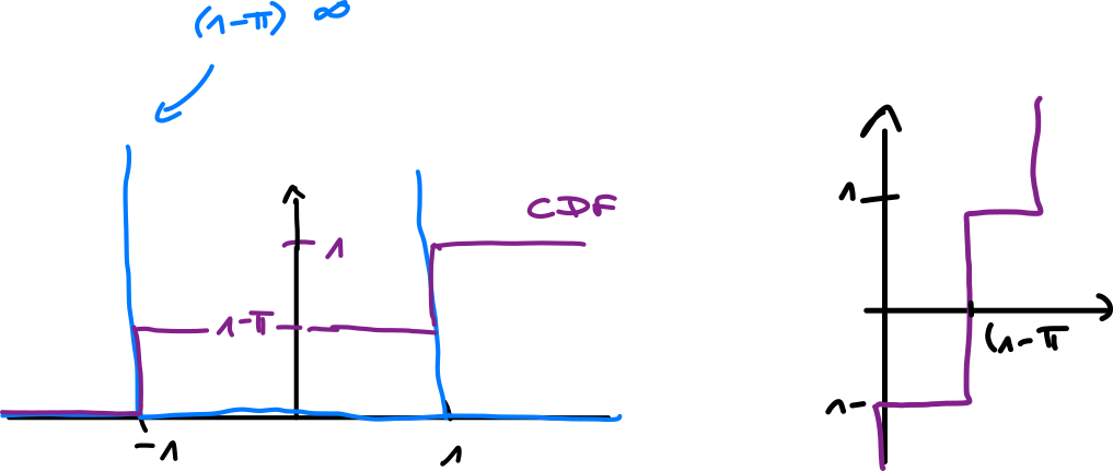
• for that, we get $\forall Z \in \left[0, 1\right]$ and so the CDF is $$f(X) = \int_{\infty}^{X} p(X)\;dx$$
• if $x \le x_{\text{min}}$ then $f(x) = 0$ (integral over nothing)
• if $x \ge x_{\text{max}}$ then $f(x) = 1$ (integral over everything)
• if $x_{\text{min}} < x < x_{\text{max}}$ then $0 < f(x) < 1$ because $p(X) \ge 0$

Ex.: exponential distribution $$p(X) = \begin{cases} \frac{1}{v}e^{-x/\tau} & x \ge 0 \\ 0 & \text{otherwise} \end{cases}$$

for $\tau$ hyperparameter $v$ normalization, which has to be $$v = \int_{0}^{\infty} e^{-x/\tau} dx' = -\tau e^{-x/\tau} \mid_{x=0}^{\infty} = \boxed{\tau}$$

To get $f(x)$, we again do the integral with upper bound being $x$, getting $$\int_{0}^{x} \frac{1}{\tau}e^{-x/\tau} dx' = 1 - e^{-x/\tau}$$

To sample from it, we solve for $x$ in the equation above and get $$\boxed{f^{-1}(z) = -\tau \log(1-z)}$$ which is either inverse CDF, quanti function or the percent-point function (PPF)

There was another example of a Gaussian PDF/CDF/PPF. Unlike the exponential, it the CDF doesn’t have a closed-form solution and has to be approximated.

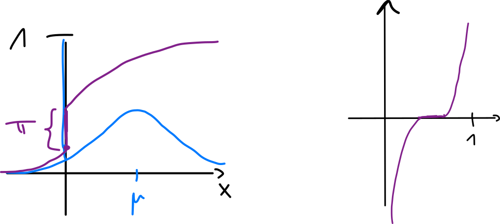
Ex.: $f(X)$ and $f^{-1}(X)$ need not be continuous (they can have jumps) – Bernoulli $$p(X) = \begin{cases} +1 & \text{probability}\ \pi \in \left[0, 1\right] \\ -1 & \text{probability}\ 1 - \pi \\ \end{cases}$$

We want to make it continuous, we do embedding via the $\delta$-distribution $$p(x) = (1 - \pi) \delta(x + 1) + \pi \delta (x - 1)$$

• the delta funtion is very handy: for any function $h(x)$, $$\int_{-\infty}^{\infty} h(x) \delta(x' - x) dx' = h(x)$$
• $\pm 1$ are atoms – their probability is not zero (unlike functions like Gaussian)

Ex.: spike-and-slab distribution $$p(X) = \begin{cases} 0 & \text{probability}\ \pi & \text{(nothing happened)} \\ \mathcal{N}(\mu, \sigma^2) & \text{probability}\ 1 - \pi &\text{(something happened)} \end{cases}$$

Classical approaches

What if we don’t know $p^*(x)$ but we have a $TS = \left\{X_i \sim p^*(X)\right\}_{i=1}^N$?

1. histogram – define $X_{\text{min}} = \min_{i} X_i$ (smallest value), $h = \frac{2\ \mathrm{IQR}(TS)}{\sqrt[3]{N}}$ (bin width)
   • the $\mathrm{IQR}(TS)$ “inter-quantile range” is obtained by sorting TS and getting the difference between values $X\left[\frac{N}{4}\right]$ and $X\left[\frac{3N}{4}\right]$ (i.e. quarter to the left, quarter to the right)
   • the formula gives a good balance between number of bins vs. the number of items per bin $$\mathrm{bin}_l = \left\{x_i: x_{\text{min}} + (l - 1)h \le x_i < x_{\text{min}} + lh\right\} \qquad N_l = \# \mathrm{bin}_l$$ $$\boxed{p(X) = \sum_{l = 1}^{L} \mathrm{1}\left[X \in \mathrm{bin}_l\right] \cdot \frac{N_l}{N \cdot h}}$$
2. generalization of a histogram – mixture distribution
   • idea: express a complicated $p(X)$ as a superposition of $L$ simple $p_l(X)$, i.e. $$p(X) = \sum_{l = 1}^{L} \pi_l p_l(X)$$
     • $\pi_l$ is weight, $p_l$ is some simple distribution
     • $\pi_l \ge 0, \sum_{l = 1}^{L} \pi_l = 1$ (has to be a probability distribution…)
   • for histogram, $p_l(X)$ is uniform
   • for Gaussians, we have Gaussian mixture model (GMM); solved with the EM algorithm
3. kernel density estimation $p_l(X) = \mathcal{N}(\mu_l, \sigma^2\mathbb{I})$ (or any other simple distribution)
   • $L = N$ (one component per training sample)
   • $\mu_l = X_l, \pi_l = \frac{1}{N}$
   • similar to mixture distribution (has less distributions), here $\sigma^2$ is the hyperparameter

Warmed up: more dimensions!

Extensions of classical approaches

1. multi-variate standard normal $$p(X) = \mathcal{N}\left(\mu=0, \Sigma=\mathbb{I}\right) = \frac{1}{\left(2\pi\right)^{D/2}}\mathrm{exp}\left(-\frac{X X^T}{2}\right)$$
   • can be expressed as a product of 1-D normal distributions: $$X X^T = \sum_{i = 1}^{D} x^2_i \implies \mathrm{exp}\left(-\frac{X X^T}{2}\right) = \mathrm{exp}\left(-\frac{\sum_{i} X_i^2}{2}\right) = \prod_{i = 1}^{D} \mathrm{exp}\left(-\frac{x_i^2}{2}\right)$$
   • $\Rightarrow$ sampling in $D$ dimensions boils down to many samplings in 1-D
2. multi-variate Gaussian distribution with mean $\mu$, covariance $\Sigma$ $$p(X) = \mathcal{N}(\mu, \Sigma) = \frac{1}{\sqrt{\det 2\pi \Sigma}} \mathrm{exp}\left(-\frac{\left(X-\mu\right)\Sigma^{-1}\left(X - \mu\right)^T}{2}\right)$$
   • to sample, we compute the eigen decomposition of $\Sigma = U \Lambda U^T$ (for $U \in \mathbb{R}^{D \times D}$ orthonormal and $\Lambda$ diagonal with eigen values) and do the following:
     • invert $\Sigma^{-1} = U \Lambda^{-1} U^{T}$ (inverse is transposition for orthogonal)
     • then $\Lambda^{-1/2} = \begin{pmatrix} \frac{1}{\sqrt{\lambda_1}} & & \\ & \ddots & \\ & & \frac{1}{\sqrt{\lambda_D}} \end{pmatrix}$
     • define new coordinates $\tilde{X} = \left(X - \mu\right) \cdot U \Lambda^{-1/2}$
     • then $\tilde{X}\tilde{X}^T = \left(X - \mu\right) \Sigma^{-1} \left(X - \mu\right)^T$
   • we can sample $D$ 1-D gaussians and put them in the $\tilde{X}$ vector, which we invert
     • $X =\tilde{X} \Lambda^{1/2} U^T + \mu$: reparametrization trick (from arbitraty Gaussian to std. normal)
   • in our language: $$Z = \left(X - \mu\right) U \Lambda^{-1/2} \sim \mathcal{N}(0, \mathbb{I}) \implies X = f^{-1}(Z) = Z \Lambda^{1/2} U^T + \mu \sim \mathcal{N}(\mu, \Sigma)$$

• similar for other analytic multi-variate distributions (scipy.stats offers ~16)

What if $p(X)$ must be learned?

Mixture model idea naturally generalizes to $D$ dimensions:

1. histograms are defined by a regular grid with $K$ levels per dimension $\implies L = k^D$ (exponential, does not scale)
   • solution: define bins by recursive subdivision (eg. density tree)
   • quality of the models is only medium – each subdivision doubles the number but looks at only one variable, which is bad if you have 100s of variables… the number of coorelations to be considered is bounded by tree depth, which must be $\mathcal{O}\left(\log N\right)$
2. for Gaussians, we have to learn co-variance (instead of variance) $\implies$ change the EM algorithm accordingly
3. kernel density estimation is also unchanged, but finding a bandwidth $\sigma^{2}$ that works equally well $\forall X_i$ is very difficult

• (2.) and (3.) become more expensive for growing $D$
  • $\mathrm{GMM} = \mathcal{O}\left(L \cdot D^2\right)$
  • $\mathrm{KDE} = \mathcal{O}\left(N \cdot D\right)$
• sampling is simple: sample $l \sim \mathrm{discrete}(\pi_1, \ldots, \pi_L)$, sample $X \sim p_l(X)$

Reducing $p(X)$ to many 1-D distributions

• naive: $p(X) = \prod_{i=1}^{D} p_j(X_j)$, learn a 1-D model for each coordinate $X_j$
  • assumes variable indepence, we loose all coorelation (highly unrealistic)

• exact: auto-regressive model – decompose $p(X)$ by Bayesian chain rule: $$p(X) = p_1(X_1) p_2(X_2 \mid X_1) p_3(X_3 \mid X_1, X_2) \ldots$$
  • any ordering of the chain rule also works (variable order is interchangeable)
  • each $p_i(X_j \mid X_{<j})$ is a collection of 1-D distributions (one distribution per value of $X_{<j}$)
    • $\Rightarrow$ use conditional inverse transform method $$x_j \sim p(X_j \mid X_{<j}) \iff z_j = p(z_j)\ ,\quad x_j = f^{1}_j (z_j ; X_{<j})$$
    • then $$f^{-1}(X) = \begin{pmatrix} x_1 = f^{-1}_1(z_1) \\ x_2 = f^{-1}_2(z_2; x_1) \\ \vdots \\ x_D = f^{-1}_D(z_D; x_1, \ldots, x_{D-1}) \\ \end{pmatrix}$$ which is auto-regressive (values rely on the previous ones)
• problem: $f_j^{-1} (z_j; x_{<j})$ is a different 1-D function for each value of $X_{<j}$
  • eg. if $X_{<j}$ is defined on a regular grid with $k$ levels per dimension, then we have $k^{j-1}$ different values $\implies$ does not scale
  • general solution: learn $f_j^{-1}$ with a neural networks
    • generalizes from a few seen (TS) values of $X_{<j}$ to all possible values
  • simpler solution: if $X_j \perp X_{j' < j}$ (independent) then $X_{j'}$ can be dropped
    • also, if $X_j \perp X_{j''} \mid X_{j'}$ for $j', j'' < j$ then $X_{j''}$ can be dropped
    • repeat with more complicated conditions, dropping as many as possible
  • example: Markov chain: $X_j \perp X_{j'} \mid X_{j-1}\ \forall j' < j - 1$ – the DAG becomes a chain
    • typical if $j$ is a timestep (future only depends on the present, not the past)
    • $f_{j}^{-1} (z_j, X_{j-1}) \forall j \implies$ easy to learn
  • example: causal model $p(X) = \prod_{j=1}^{D} p_j(X_j \mid \mathrm{PA}(X_j))$ for $\mathrm{PA}$ causal parents of $x_j$
    • e.g. both earthquake and burglar cause the alarm (not the other way lmao)
    • causal DAG has the fewest edges (i.e. easier to learn) BUT finding it is very hard

Measuring model quality

• we can measure “distance” between $p(X)$ and $p^*(X)$ (even if we don’t know $p^*(X)$) to:
  1. use as objective function for training
  2. use for validation after training

Forward KL divergence

$$\mathrm{KL}\left[p^* \mid\mid p\right] = \int p^*(X) \log \frac{p^*(X)}{p(X)}\ dx = \mathbb{E}_{\underbrace{x \sim p^*(X)}_{\text{forward}}} \left[\log \frac{p^*(X)}{p(X)}\right]$$

A few useful properties:

• $\mathrm{KL}\left[p^* \mid\mid p\right] = 0 \iff p^*(X) = p(X)$
• $\mathrm{KL}\left[p^* \mid\mid p \right] \ge 0$

It’s a divergence and not a distance (i.e. a metric) – not symmetric, triangular inequality doesn’t hold

There was an example here with a discrete distribution.

Caveat: if there are datapoints in $X$ s.t. $p^*(X) > 0$ but $p(X) = 0$, then $\mathrm{KL} = \infty$

• $\Rightarrow$ can’t be used as training gradient (since it’s infinity)
• $\Rightarrow$ use model families s.t. $\mathrm{dom}(p^*(X)) \subseteq \mathrm{dom}(p(X))$

Relationship between forward KL and maximum likelihood training: $$\mathrm{KL}\left[p^* \mid \mid p\right] = \underbrace{\int p^*(X) \log p^*(X) dx}_{H\left[p^*\right] \text{(entropy)}} - \underbrace{\int p^*(X) \log p(X) dx}_{\mathbb{E}_{X \sim p^*(X) \left[-\log p(X)\right]}}$$

• entropy is independent of $p(X)$ and can be dropped, so get an optimization problem $$\hat p(X) = \argmin_{p(X) \in \mathcal{f}} \mathbb{E}_{X \sim p^*(X)} \left[-\log p(X)\right]$$
  • minimize KL $\iff$ minimize NLL $\iff$ maximize $p(X)$ for $TS$

Given $TS = \left\{X_i \sim p^*(X)\right\}_{i=1}^N$, $$\boxed{\hat p(X) \approx \argmin_{p(X)} \frac{1}{N} \sum_{i=1}^{N} -\log p(X_i)}$$

• does not contain $p^*(X) \implies$ we can optimize without knowing $p^*(X)$ (samples sufficient)
• but we need to calculate $p(X_i)$ during training $\implies$ must be capable to do “inference”

Reverse KL divergence

$$\mathrm{KL}\left[p \mid\mid p^*\right] = \int p(X) \log \frac{p(X)}{p^*(X)}\ dx = \mathbb{E}_{\underbrace{x \sim p(X)}_{\text{reverse}}} \left[\log \frac{p(X)}{p^*(X)}\right]$$

• empirical approximation: iterate $t = 1 \ldots T$:
  • current guess $p^{(t-1)}(X)$: draw batch $\left\{X_i \sim p^{(t-1)} (X)\right\}_{i=1}^N$
  • $p^{(t)}(X) \argmin_{p(X)} \frac{1}{N} \sum_{i=1}^{N} \log \frac{p(X_i)}{p^*(X_i)}$
    • $\Rightarrow$ need to know $p^*(X)$… cannot be used in many application
    • useful when we know the distribution but it’s intractable (ex. Gibbs distribution)

Comparison (forward x reverse)

• forward KL tends to smooth out models of $p^*(X)$ – mode-covering
• reverse KL tends to focus on single (or few) highest modes – mode-seeking/collapse

Maximum Mean Discrepancy

The idea is to use the kernel trick

• without kernel:
  • define $\varphi: \mathrm{dom}(X) \implies \mathbb{R}$
  • two data sets $\left\{X_i^* \sim p^*(X)\right\}_{i=1}^N, \left\{X_i \sim p(X)\right\}_{i=1}^M$
  • calculate $\tilde X_i = \varphi(X_i), \tilde X_i^* = \varphi(X_i^*)$ $$\mathrm{MMD} = \max_{\varphi \in \mathcal{F}} \left[\frac{1}{M} \sum_{i=1}^{M} \varphi(X_i) - \frac{1}{N} \sum_{i=1}^{N} \varphi (X_i^*)\right]$$
    • $\mathrm{MMD} \ge 0$ (if $-\varphi \in \mathcal{F}$ when $\varphi \in \mathcal{F}$)
    • $\mathrm{MMD} = 0 \iff p(X) = p^*(X)$
    • $\mathrm{MMD}$ is a metric
  • $\varphi$: witness function – certifies that $p$ and $p^*$ are different when $\mathrm{MMD}$ is big
    • family function $\mathcal{F}$ must be chosen s.t. we can’t cheat (i.e. arbitratily add/multiply to increase – e.g. conditions on variance)
• now replace explicit mapping $\varphi(X)$ with a kernel function $k(X, X')$: $$\begin{aligned} \mathrm{MMD}^2 &= \frac{1}{M(M-1)} \sum_{i=1}^{M} \sum_{i' \neq i} k(X_i, X_{i'}) \quad //\ \text{repulsion between synthetic $X_i$} \\ &+ \frac{1}{N(N - 1)} \sum_{i=1}^{N} \sum_{i' \neq i} k(X_i^*, X_{i'}^*) \quad //\ \text{independent of $p(X)$} \\ &- \frac{2}{M N} \sum_{i=1}^{M} \sum_{i'=1}^{N} k(X_i, X_{i'}^*) \quad //\ \text{attraction between synthetic and real}\end{aligned}$$

Typical kernels (for $h, L$ hyperparameters):

• squared exponential $$k(X, X') = \mathrm{exp}\left(- \frac{||X - X'||^2}{2h}\right)$$
• inverse multi-quadratic $$k(X, X') = \frac{1}{\frac{||X - X'||^2}{h} + 1}$$
• multi-scale squared exponential $$k(X, X') = \sum_{l=1}^{L} \mathrm{exp}\left(- \frac{||X - X'||^2}{2h_l}\right)$$

Generative Modeling with NN

• relationship between generative modeling and compression: both are essentially $$X \rightarrow f(X) \rightarrow Z \rightarrow q(Z) \rightarrow \hat X$$
  • lossless: $\hat X = X$ (e.g. ZIP)
    • idea: use short codes for frequent symbols and longer for more rare symbols
  • lossy compression: $\hat X \approx X$ (e.g. JPEG)
    • idea: decompose into smaller parts, drop important stuff, use lossless compression for important stuff

Here we have 3 conflicting goals:

1. small codes: $d = \mathrm{dim}(Z) \ll \mathrm{dim}(X) = D$
2. accurate reconstruction: $\mathrm{dist}(X, \tilde X) \approx 0$ (for some distance function)
3. preserve data distribution: $\mathrm{dist}(p^*(X), p(\hat X)) \approx 0$ (for some distribution)

Note that $3 \not\Rightarrow 2$ (shown during lecture).

Autoencoder

• learned compression: $f(X)$ and $q(Z)$ are neural networks
  • lossy compression because usually $d < \dim(Z) \ll \dim(X) = 1$
    • “bottleneck” is a hyperparameter
  • train by reconstruction error $$\hat f, \hat g = \argmin_{f, g} \mathbb{E}_{X \sim p^*(X)} \left[||X - q(f(X))||^2\right]$$
• distance functions for the loss:
  • $L_2$ is most common
  • $L_1$ tends to be less blurry for images (better preserves small details)
  • multi-resolution $L_p$: compute image pyramid (apply loss to different image sizes)
• denoising autoencoder: add more noise to the data to teach the network what noise is $$\tilde X = X + \varepsilon \quad \varepsilon \sim \mathcal{N}(\varepsilon \mid 0, \sigma^2 \mathbb{I})$$ $$\hat f, \hat g = \argmin_{f, g} \mathbb{E}_{X \sim p^*(X), \varepsilon \sim \mathcal{N}(\varepsilon \mid 0, \sigma^2 \mathbb{I})} \left[||X - q(f(X + \varepsilon))||^2\right]$$
  • better, deep mathematical properties later
• autoencoder is not a generative model (according to our definition):
  1. we haven’t learned the distribution – no generative capability
  2. no inference, i.e. no way to calculate $p(X)$

Generating data

1. expert learning of $p_E(Z)$ by a second generative model
   • often simpler than learning $p^*(X)$ directly (e.g. $d < D$)
   • Stable Diffusion (image generation) does this
2. joined optimization:
   • predefine $q(Z)$ (desired code dimension)
   • measure $\mathrm{MMD}\left(p_E(Z), q(Z)\right) \implies$ add new loss term
     • choosing a kernel is another hyperparameter $$\hat f, \hat g = \argmin_{f, g} \mathbb{E}_{X \sim p^*(X)} \left[||X - q(f(X))||^2\right] + \lambda \mathrm{MMD}\left(f_\#p^*, q\right)$$
   • paper: variant of INfoVAE [2019]
3. variational autoencoder (VAE) [2014]
   • idea: replace deterministic functions $f(X)$ and $q(Z)$ with conditional distributions
     • encoder: $p_E(Z \mid X)$, decoder $p_D(X \mid Z)$
     • we also have data $p^*(X)$ and desired code dist. $q(Z)$
   • implies two version of joint distribution of $X$ and $Z$
     • encoder $p_E(X, Z) = p^*(X) \cdot p_E(Z \mid X)$ (Bayes)
     • decoder $p_D(X, Z) = q(Z) \cdot p_D(X \mid Z)$ (also Bayes)
   • two requirements:
     1. decoder marginal $p(X) = \int p_D(X, Z)\;dz \approx p^*(X)$
     2. encoder-decoder pair must be self-consistent: $p_E(X, Z) = p_D(X, Z)$
   • here we will use the $\mathrm{ELBO}$ loss: $$\mathrm{ELBO} = \underbrace{-\mathrm{KL}\left[p_E(Z \mid X) \mid\mid q(Z)\right]}_{\text{how close is $p_E(Z \mid X)$ to $q(Z)$}} + \underbrace{\mathbb{E}_{p_E(Z \mid X)} \left[\log p_D(X \mid Z)\right]}_{\text{reconstruction error}}$$
     • trade-off between two objectives:
       • reconstruction error minimized if encoder & decoder are deterministic with perfect reconstruction
       • first term minimized if $p_E(Z \mid X) = q(Z)$ – encoder ignores the data, which is the opposite of perfect reconstruction
   • maximizing $\mathrm{ELBO}$ loss enforces (2) (proved during the lecture)
     • in literature, $\mathrm{ELBO}$ is usually maximized
     • conceptually, minimizing $-\mathrm{ELBO}$ is simpler
   • maximizing the $\mathrm{ELBO}$ also indirectly maximizes the data likelihood under the model – ML principle: TS should be a typical model outcome
     • $\iff$ minimize expected negative log-likelihood (NLL) (proved during the lecture)
     • $-\mathrm{ELBO}$ is an upper bound for NLL loss
   • most common implementation encoder and decoder are diagonal Gaussians: $$p_E(Z \mid X) = \mathcal{N}(Z \mid \mu_E(X), \mathrm{Diag}(\sigma_E(X)^2))$$ $$p_D(X \mid Z) = \mathcal{N}(X \mid \mu_D(Z), \beta^2 \mathbb{I})$$
     • since we only have diagonal Gaussians, we can’t rotate the ellipses
     • since we only have Gaussians, the shape is restricted to circles
     • if $q(Z) = \mathcal{N}(0, \mathbb{I})$ then $\mathrm{KL}\left[p_E \mid\mid g\right]$ can be calculated analytically
     • if $p_D(X \mid Z) = \mathcal{N}(Z \mid \mu_D(Z), \beta^2 \mathbb{I})$, reconstruction error becomes squared loss
     • $\beta^2 \gg 1$ downscales squared loss $\implies$ reconstruction error unimportant
     • $\beta^2 \ll 1$ upscales squared loss $\implies$ reconstruction error dominant
     • generation: $Z \sim q(Z), X \sim p_D(X \mid Z) \iff \mu_D(Z) + \overbrace{\beta^2 \varepsilon}^{\text{noise}}$
     • inference: if $p(X) = p^*(X)$ and $p_E(X, Z) = p_D(X, Z)$ then $$p_E(X, Z) = p(X) p_E(Z \mid X) = q(Z) p_D(X \mid Z) = p_D(X, Z)$$ $$\implies p(X) = \frac{q(Z) p_D(X \mid Z)}{p_E(Z \mid X)}$$ must give the same value for all $Z \sim p_E(Z \mid X)$
4. conditional VAE
   • instead of learning $p(X)$, we learn $p(X \mid Y)$ for some variable $Y$
   • e.g. $Y \in \left\{0, \ldots, 9\right\}$ for MNIST label $$p(X \mid Y) = \int q(Z) \cdot p_D (X \mid Y, Z)\;dz \implies p(X) = \sum_{Y} p(X \mid Y) p^*(Y)$$
   • if encoder & decoder are Gaussians, add $Y$ as input to the networks
   • we can supply different labels for encoding / decoding – style transfer
     • one digit in style of another / one image in the style of another
   • here we can do operative classification: test $X$ with unknown label, try encoding with every label and calculate the corresponding $p(X \mid Y)$, returning the one with maximum probability

Generative Adversarial Networks (GANs)

• dominant generative model 2014-2019/20
  • now diffusion models and transformers are better
• idea: learn quality function (instead of hand-crafted formula like MMD)
  • new NN “discriminator/critic” $C$ – classifier $p(X\ \text{is real} \mid X)$ vs. $p\left(X \text{is fake} \mid X\right)$
  • train the decoder (“generator”) jointly with the critic
• training becomes a game:
  • critic becomes better at distinguishing reals and fakes
  • decoder becomes better at fooling the critic
  • $\Rightarrow$ training objective $$\hat C, \hat D = \argmin_{D} \argmax_{C} \mathbb{E}_{X \sim P^*(X)} \left[\log p_C(X\ \text{is real} \mid X)\right] + \mathbb{E}_{Z \sim g(Z)} \left[\log p_C(X \text{is fake} \mid X = D(Z)) \right]$$
  • at optimal convergence, we have $p(X) = p^*(X)$ (~proven during the lecture)
    • assumes that we have a perfect critic and proves from there
  • in practice, we don’t have a perfect critic (and it wouldn’t work in practice because for the bad decoder, recognizing fakes is easy so gradient will be zero and we won’t train anything)
    • instead, train $D$ and $C$ jointly (both random initially) via alternating optimization – one step for $D$, one/more steps for $C$
    • also use non-saturating loss – replace $\log(1 - p(\text{real} \mid X))$ with $-\log(p(\text{real} \mid X))$
      • global optimum is preserved, should work better for training
      • see the graphs for $-\log(X)$ vs. $\log(1 - X)$ $$\hat C = \argmin_C \mathbb{E}_{X \sim p(X)} \left[\log p_C(\text{real}\mid X)\right] + \mathbb{E}_{Z \sim g(Z)} \left[\log (1 - p_C(\text{real}\mid D(Z)))\right]$$ $$\hat D = \argmin_D \mathbb{E}_{Z \sim g(Z)} \left[-\log p_C(\text{real}\mid D(Z))\right]$$
• GANs defined state-of-the-art up to 2019/20:
  • WassersteinGAN: uses alternative loss for critic (not really better)
  • CycleGAN: replace $g(Z)$ with true distribution over another variant of real data
    • e.g. $p^*(X)$ dist. of daylight photos, $\tilde p^*(\tilde X)$ dist. of night photos
    • two cases:
      1. paired dataset (same $X$ from both variants) – supervised learning
      2. unpaired dataset (no overlap between instances)
    • we have new “cycle losses” – $||X - D(E(X))||^2$ and $||\tilde X - E(D(\tilde X))||^2$ should be small
    • for paired, we additionally have $||\tilde X_i - E(X_i)||^2$ and $||X_i - D(\tilde X_i)||^2$
    • we still need a critic, otherwise $D$ and $E$ are identity (must combine with cycle loss)
    • as opposed to GAN, we have no bottleneck – $X$ and $\tilde X$ are the ~same dimensions
  • InvertibleGAN: add an encoder to original GAN
    • recreating codes $Z(X)$ and distinguishing reals from fakes can use the same image features $\implies$ same network to encode and decode
    • $+$ many more additional losses (similar to CycleGAN)
    • $-$ hyperparameter optimization is hard

Normalized Flows (NF)

• one of the major recent approaches

Goals	Autoencoder	VAE	GAN	NF
small codes	hyperp.	hyperp.	hyperp.	lossless
accurate distribution $$p(X) \approx p^*(X)$$	bad (doesn’t care)	trade-off	good	good
good reconstruction $$\hat X = D(E(X)) \approx X$$	good	trade-off	can’t	good

Idea: generalize the inverse transformation method to arbitrary dimensions:

• $X \in \mathbb{R}^D, p^*(X)$ high-dimensional density, $A \in \mathbb{R}^D$ a region
• define $\mathrm{Pr}[X \in A] = \int_{A} p^*(X)\;dx$
• let $Z = f(X)$ an invertible encoding, $X = f^{-1}(Z) := g(Z)$
• $\tilde A = f(A)$ the image of $A$ in $Z$-space: $$\tilde A = \left\{Z: Z=f(X)\ \text{for}\ X \in A\right\}$$
• we want consistency: for all $$A: \mathrm{Pr}[Z \in \tilde A] = \int_{\tilde A} q(Z)\;dz \overset{!}{=} \mathrm{Pr}\left[X \in A\right]$$
• apply the multi-dimensional change-of-variables formula: $$\int_{\tilde A = f(A)} q(Z)\;dz = \int_{q(\tilde A)} q(Z=f(X))\; | \det \mathcal{J}_{f} |\;dx$$ for the Jacobian (matrix of partial derivatives) $\mathcal{J}_f$ of $f$

Since consistency must hold for any $A$, the integrals must be equal, we get the multi-variate change-of-variables formula $$\boxed {p(X) = q(Z = f(X))\; | \det \mathcal{J}_f (X) | }$$

Goal:

• pre-define $q(Z)$, e.g. $q(Z) = \mathcal{N}(0, \mathbb{I})$
• learn $f(X)$ s.t. $p(X) \approx p^*(X)$ ($f(X) \cong$ neural network)

Recall the $1$-D case: $q(Z) = \text{uniform}(0, 1) \implies f(X) = \mathrm{CDF}_{p^*}(X)$

• for learning $q(Z) = \mathcal{N}(0, \mathbb{I})$ is better:
  • has non-zero gradients for gradient descent
  • supported on all of $\mathbb{R}^D$ (unlike uniform – what to do with points outside?)

Two difficult problems in practice, covered in the next sections:

1. how to ensure that $f(X)$ is invertible & efficiently compute $f^{-1}(Z)$
2. how to (efficiently) calculate $\det \mathcal{J}_f$

(2) Calculating $\det \mathcal{J}_f$

• 2-D case is easy: $$\det \begin{pmatrix} a & b \\ c & d \end{pmatrix} = ad - bc$$
• for higher cases, we can calculate determinants recursively, which grows exponentially
• general solution with SVD: $\mathcal{J} = U \cdot \Lambda \cdot V^T \implies |\det \mathcal{J}| = |\det \Lambda| = \prod_j \lambda_j$
  • effort of $\mathcal{O}(D^3)$, which is a little better than exponential
• we can also expoit special case if $\mathcal{J}$ is triangular (and the diagonal is non-zero, otherwise the determinant is zero), in which case $\det \mathcal{J}$ is just the product of the diagonal elements
  • we already talked about an instance of this: auto-regressive models – since they rely on the previous terms, the Jacobian is triangular and the determinant is very easy

If $f(X)$ is a multi-layer network, $f(X)$ is a composition of functions $f^{(l)}$

• the Jacobian of comosition is the product of all Jacobians (consequence of chain)
• the determinant is the product of determinants (consequence of linear algebra)
• $\Rightarrow$ determinant of multi-layer network is easy when layer determinants are
• $\Rightarrow$ popular architecture is to define all $f^{(l)}\left(Z^{(l-1)}\right)$ as auto-regressive functions

(1) Ensuring that $f(X)$ is invertible and computable

• trick: chose $f^{(l)}$ auto-regressive and easy to invert
• major architecture: Coupling layer $\implies$ network is “real NVP” (non-volume-preserving due to the determinants being non-unit)
  • auto-regressive model
  • in each layer, change only half of the dimensions of $Z^{(l-1)}$
  • pass the remaining dimensions on unchanged (“skip connection”) $$\begin{aligned} Z_{j}^{(l)} &= Z_{j}^{(l-1)} \; &&\forall j=1, \ldots, \tilde D \quad \text{for}\ \tilde D = \left\lfloor D/2 \right\rfloor \\ Z_j^{(l)} &= f_j^{(l)} \left(Z_j^{(l-1)}, Z_{1:\tilde D}^{(l-1)}\right) \; &&\forall j = \tilde D + 1, \ldots, D \end{aligned}$$ $$\mathcal{J}^{(l)} = \begin{pmatrix} \mathrm{I}_{\tilde D} & \mathrm{0}_{\tilde D} \\ \neq 0 & \mathrm{diag}\left(\frac{\partial f_j^{(l)}}{ \partial Z_j^{(l-1)}}\right) \\ \end{pmatrix}$$
  • no surprise since it’s a variant of the auto-regressive model $$\boxed{\det \mathcal{J}^{(l)} = \prod_{j=\tilde D}^{D} \frac{\partial f_j^{(l)}\left(Z_{j}^{(l-1)}, Z_{\le \tilde D}^{(l-1)}\right)}{\partial Z_{j}^{(l-1)}}}$$
• simplest invertible function – affine functions: $Z_{j}^{(l)} = s \cdot Z_j^{(l-1)} + t$
  • $s$ and $t$ are neural networks that we train: $s_j^{(l-1)}\left(Z_{\le \tilde D}^{(l-1)}\right)$ (same for $t$)

TODO: add the drawing here

• for $f^{(l)}_j$ to be invertible, we need $s^{(l)}_{j} \neq 0$
  • $\Rightarrow$ we actually learn $\tilde s_j^{(l)}$ and set $s_j^{(l)} = \exp(\tilde s_j^{(l)}) > 0$
    • also takes care of the sign of the Jacobian – no abs!
    • in practice, it is numerically more stable to set $s_j^{(l)} = \exp(\tanh(\tilde s_j^{(l)}))$

Summary

• forward: $$\begin{aligned} Z_j^{(l)} &= \exp\left(\tilde s_{j}^{(l)}\left( Z_{\le \tilde D}^{(l-1)}\right) \right) Z_j^{(l-1)} + t_j^{(l)}\left(Z_{\le \tilde D}^{(l-1)}\right) \quad j > \tilde D \\ Z_j^{\left(l\right)} &= Z_j^{(l-1)} \quad j \le \tilde D \end{aligned}$$
• inverse: $$\begin{aligned}Z_j^{\left(l-1\right)} &= Z_j^{\left(l\right)} \quad j \le \tilde D \\ Z_j^{\left(l-1\right)} &= \left(Z_j^{\left(l\right)} - t_j^{\left(l\right)}\left(Z_{\le \tilde D}^{\left(l-1\right)}\right)\right) \cdot \exp \left(-\tilde s_j^{\left(l\right)} \left(Z_{\le \tilde D}^{\left(l-1\right)}\right)\right) \quad j > \tilde D \end{aligned}$$
• $\Rightarrow$ invertible layer constructed from non-invertible $s$ and $t$

• $\Rightarrow$ choose $s$ and $t$ according to architecture (fully-connected, convolutional, etc.)

• determinant of an affine coupling layer $$\det \mathcal{J}^{(l)} = \text{boxed equation above} = \prod_{j=\tilde D + 1}^{D} \exp \left(\tilde s_j^{(l)} \left(Z_{\le \tilde D}^{(l-1)}\right)\right)$$

RealNVP

• invertible NN with autoregressive form, i.e. $\det \mathcal{J}_f$ is easy
• after each coupling layer apply orthonormal transformation $Q$, e.g. permutation
  • have $| \det(Q) | = 1$ and $Q^{-1} = Q^T$ so easy to work with
• it turned out experimentally that learning $Q$ is not necessary, no one knows why
  • fixed matrices are sufficient / may change with new learning algorithm
• final architecture: $$f = f^{(L)} \circ Q^{(L - 1)} \circ f^{(L - 1)} \circ \ldots \circ Q^{(1)} \circ f^{(1)}$$
• training algorithm: minimize negative likelihod of data (derivation in slides): $$\boxed{\hat f = \argmin_f \frac{1}{N} \sum_{i=1}^{N} \left(\frac{f(X_i)^2}{2} - \sum_{l=1}^{L} \sum_{j=\tilde D + 1}^{D} \tilde s_{j}^{(l)} \left(Z_{i, 1:\tilde D}^{(l-1)}\right)\right)}$$
• the slides here explain why affine coupling works

Spline coupling

• better than affine coupling for low dimensions ($D < 20$)
• uses Hermite splines, which require location of knots, function at knots and derivatives at knots (with interpolation in between)
• most popular: rational quadratic spline [Neural Spline Flows, 2019]

Conditional derivatives

• e.g. $Y$ is digit label, $X$ is MNIST
  • $X \sim p(X)$: sample any digit
  • $X \sim p(X \mid Y = Z)$: sample only $2$s
• typical setup for supervised learning:
  • traditional networks point estimates $\hat X = r(Y)$ (regression or classification)
  • conditional NFs: distribution of $X \hat=$ estimate uncertainty of $X$
• an autoregressive function is easy to generalize for conditionality: $$Z = f(X; Y) = \begin{pmatrix} f_1(X_1; Y) \\ f_2(X_2; X_1; Y) \\ \vdots f_D(X_D, X_{1:D-1}, Y) \end{pmatrix}$$
  • $Y$ can be added as an input to all nested networks $s^{(l)}, t^{(l)}$
  • works if $Y$ is known for both forward and backward network execution
• if $Y$ is complicated (e.g. high dimensional image), we have shared preprocessing network $\tilde Y = h(Y)$ (feature detector / summary network), which can
  • use architecture of an existing regression networks minus the last layer
  • use a foundational model $\phi(Y)$ trained by the big guys on big data

Simulation-based inference (SBI)

• setting:
  • $X$ is observables, i.e. variables we can measure
  • $Y$ are hidden properties, i.e. variables we’d like to know but can’t measure
• assumptions:
  1. hidden variables are more fundamental, e.g. $Y$ is caused by $X$
  2. we have a scientific theory how the $X$ arrise from the $Y$ (forward process)
  3. theory is implemented as an algorithm $\hat=$ computer simulation
     • $\Rightarrow$ we can do “in-silico experiments” (as opposed to “in-vivo” and “in-vitro”)
     • three types of variables:
       • $Y$: inputs to the simulation (pretend we know the hidden state)
       • $X$: outputs
       • optionally $\eta$: random variables for non-deterministic simulation
       • deterministic $X = \phi(Y)$ (the simulation program) $\Rightarrow p^{S}(X \mid Y) = \delta(X - \phi(Y))$
       • non-deterministic $X = \phi(Y, \eta)$ – “noise outsourcing” $\Rightarrow p^S(X \mid Y) = \phi_{\#}p^S(Y, \eta)$
• simulation paradigm: if we knew $Y$, we could predit $X$
  • since we don’t know $Y$, try multiple $Y$ and generate alternate scenarios
    • during covid, get various assumptions about the virus and about prevention measures ($Y$) and simulate what happens ($X$), getting various scenarios
  • it’s hard to select a good set of $Y$s – SBI improves upon this
• two important special cases of the structure of $Y$:
  1. mixed effects model $$Y = \begin{cases} Y_G & \text{global properties (same for all members)} \\ Y_L & \text{local properties (differs for all members)} \\ \end{cases}$$
     • $Y_G \sim p^S(Y_G))$
     • for $i=1, \ldots, N$, sample $Y_{Li} \sim p^S(Y_L \mid Y_G)$ and $X_i \sim p^S(X \mid Y_G, Y_{Li})$
     • look at the group first, then differentiate for each individual
     • $X_i \not\perp X_{i'}$, but $X_i \perp X_{i'} \mid Y_G$ (independent conditionally based on the global assumptions)
  2. dynamical systems (time-dependent behavior) $$Y = \begin{cases} Y_G & \text{global properties (don't change over time)} \\ S_t & \text{hidden state at time $t$} \\ \end{cases}$$
     • $Y_G \sim p^S(Y_G))$
     • $S_0 \sim p^S(S_0 \mid Y_G)$
     • for $i=1, \ldots, T: S_t \sim p^S(S \mid Y_G, S_{<t})$, $X_t \sim p^S(X \mid Y_G, S_{\le t})$
     • look at the group first, then differentiate for each individual
     • if $t$ is continuous, we get a stochastic differential equation
     • if $t$ is discrete, we get a hidden Markov model
     • $X_t \not\perp X_{t'}$, but $X_t \perp X_{t'} \mid S_t$ (if Markov property is fulfilled) \end{cases}]

Main tasks of SBI

1. surrogate modelling: train a model $p(X \mid Y)$ that emulates the simulation
   • good for speed-up (since $X = \phi(Y, \eta)$ is often slow)
   • forward inference: often, $X = \phi(Y, \eta)$ only defines $p^S(X \mid Y) = \phi_{\#} (Y, \eta)$ implicitly, but doesn’t allow to calculate $p^{S}(X=X \mid Y)$ (“likelihood-free inference, implicit likelihood”)
     • approximate true likelihood by $p(X \mid Y) \approx p^S(X \mid Y)$
2. inverse inference: run the simulation backwards: $Y = \phi^{-1}(X)$
   • usually intractable (no analytic solution) and/or ill-posed (no inverse)
   • traditional solution would be to pick constrainst & regularization that select one
   • SBI solution: pick probabilistic via Bayes rule $$p^S(Y \mid X) = \frac{p^S(Y) p^S(X \mid Y)}{p^S(X)}$$
     • define equivalence classes $\mathcal{F}(X) = \left\{Y : \exists \eta \ \text{with}\ \phi(Y, \eta) = X\right\}$
       • all $Y$s that could have produced given $X$
     • posterior $p^S(Y \mid X)$ assigns a “possibility” to every $Y \in \mathcal{F}(X)$
     • problems:
       • if likelihood $p^S(X \mid Y)$ is only implicitly defined then Bayes rule canot be calculated (i.e. surrogate model above)
       • even if $p^S(X \mid Y)$ (or a surrogate) is known, Bayes rules is usually intractable
         • $\Rightarrow$ learn generative model for posterior $p(Y \mid X) \approx p^S(Y \mid X)$
3. model missclasification & outliner detection – a simulation is not reality: $$\underbrace{p^S(Y) \cdot p^S(X \mid Y)}_{\text{simulation}} \approx \underbrace{p^*(Y)p^*(X \mid Y)}_{\text{reality}}$$
   • $\Rightarrow$ use SBI to detect if $p^S(X, Y) \neq p^*(X, Y)$
   • this and observed outcome $X^{\text{obs}} \sim p^*(X, Y)$ compatible with $p^S(X, Y)$
     • if not, the simulation is unrealistic – “simulation gap”
     • is a set of outcomes $\left\{X_{i}^{\text{obs}}\right\}_{i=1}^N$ compatible with $p^S(X, Y)$?
4. model comparison and selection
   • if we have competing theories $X = \phi^{(l)}(Y^{(l)}, \eta^{(l)})$
   • $\Rightarrow$ determine which $l$ describes $X^{\text{obs}}$ best (if any)
5. digital twins: in a mixed effects setting, given $\left\{X_i^{\text{obs}}\right\}_{i=1}^N$
   • determine $Y_n$ and $Y_{Li}$ accurately enough to predict $X_i^{\text{future}} = \phi(Y_G, Y_{Li}, \eta)$
     • the same treatment that worked on this pacient will work on this one too
   • classical: base treatment decisions mainly on $Y_G$ (“treatment guidelines”) after an appropriate stratification of population into subgroups
   • desired: “precision medicine” – use $Y_G$ and $Y_{Li}$
6. experimental design and active learning: how should we measure $\left\{X_i^{\text{obs}}\right\}_{i=1}^N$ to learn as much as possible about $Y$ with given experiment budget?

Classical approaches for inverse inference

1. conjugate priors – chose $p^S(Y)$ and $p^S(X \mid Y)$ such taht $p^S(Y \mid X)$ can be analytically calculated and is in the same distribution family as $p^S(Y)$ ($\Rightarrow$ incremental Bayesian updating)
   • common is the Gaussian (surprise surprise) but exists for many other distributions
   • $+$ efficient and mathematically elegant
   • $-$ very unrealistic $\Rightarrow$ big simulation gap (usually picked for convenience)
2. likelihood-based inference – $p^S(Y)$ and $p^S(X \mid Y)$ are known (not just $X = \phi(Y, \eta)$)
   • but $p^S(Y \mid X)$ is intractable (so we can’t use Bayes rule)
   • $\Rightarrow$ create a sample $\left\{Y_n \sim p^S(Y \mid X=X^{\text{obs}})\right\}_{k=1}^K$ using Markov chain Monte Carlo (MCMC)
     • important relaxation: $p^S(X, Y)$ can be unnormalized (e.g. Gibbs distribution)
   • $+$ very general, has lots of mathematical theory
   • $+$ implemented in many libraries/languages
   • $-$ not amortized – runs from scratch for each new $X^{\text{obs}}$
   • $-$ expensive – $T$ must be very large for complete “mixing”, i.e. until all modes of $p^S(Y \mid X^{\text{obs}})$ have been covered
   • $-$ often, a long “burn-in” phase is needed to forget a bad initial guess
     • throw away $Y^{(0)} \ldots Y^{(T_0)}$
   • $-$ samples $Y^{(t)}$ and $Y^{(t-1)}$ are close to each other (chain moves slightly away from the previous guess) – may bias derived statistics of the chain (i.e. both are rejected)
     • skip each $k$th samples in the chain
   • $-$ often difficult to define proposal distribution $p(Y' \mid Y^{(t-1)})$ that has low rejection rate
   • $\Rightarrow$ only applicable when $\mathrm{dim}(Y)$ is not large and $p^S(X \mid Y)$ not too slow

Algorithm (MCMC):

1. $X^{\text{obs}}$ given, $Y^{0}$ arbitrary initial guess
   • pick a “proposal transition distribution” for transition prob $q(Y' \mid Y^{(t-1)}, X^{\text{obs}})$
     • is a hyperparameter, e.g. a Gaussian – something easy to work with
2. for $t=1, \ldots, T$
   • sample a proposal $Y' \sim q(Y' \mid Y^{(t-1)}, X^{\text{obs}})$
   • calculate acceptance weight $$\alpha = \frac{p^S(X^{\text{obs}} \mid Y') p(Y')}{p^S(X^{\text{obs}} \mid Y^{(t-1)}) p^S(Y^{(t-1)})} = \underbrace{\frac{p^S(Y' \mid X^{\text{obs}})}{p^S(Y^{(t-1)} \mid X^{\text{obs}})}}_{\text{intractable}}$$
   • sample $u \sim \text{uniform}(0, 1)$– acceptance threshold
   • if $u \le \alpha$: accept ($Y^{(t)} = Y'$), else reject ($Y^{(t)} = Y^{(t-1)}$)
     • theory: for $T \rightarrow \infty$, $\left\{Y^{(t)}\right\}_{t=1}^T \sim p^S(Y \mid X^{\text{obs}})$
3. likelihood-free inference – $p^S(X \mid Y)$ is unknown and only implicitly defined as $\phi_{\#} p^S(Y, \eta)$
   • only samples $X = \phi(Y, \eta)$ with $Y, \eta \sim p^S(Y, \eta)$
   • Approximate Bayesian Computation (ABC) $\hat =$ brute force
   • requires a distance $\mathrm{dist}(X, X^{obs})$ for outcomes, usually hand-crafted
   • $+$ works when MCMC doesn’t
   • $+$ implemented in many libraries/languages
   • $-$ very slow – if $\varepsilon$ is small, the model is more precise and slower
   • $-$ not amortized
   • $-$ hard to define $\mathrm{dist}$ if $X$ is complicated or $\mathrm{dim}(X)$ is high
     • design hand-crafted summary statistics $h(X)$ and compare $\mathrm{dist(h(X), h(X^{\text{obs}}))}$
   • $\Rightarrow$ only applicable when $\mathrm{dim}(Y)$ is not large

Algorithm (ABC):

1. $t=0$, sample $\left\{\right\}$ (we later become $\left\{Y^{(t)} \sim p^S(Y \mid X^{\text{obs}})\right\}_{t=1}^T$
2. repeat until $t=T$
   • sample $Y, \eta \sim p^S(Y, \eta)$, simulate $X \sim \phi(Y, \eta)$
   • if $\mathrm{dist}(X, X^{\text{obs}}) \le \varepsilon$, add $Y$ to samples and increase $t$, else reject
     • if we were lucky with $Y$, we accept; otherwise reject

Doing it better with NN

• amortized SBI – given $\mathrm{TS} = \left\{Y_i \sim p^S(Y), X_i = \phi(Y_i, \eta_i)\right\}_{i=1}^N, \eta_i \sim p^S(\eta \mid Y_i)$
  • noise often independent of $Y_i$ (i.e. just a random number)
  • easy to create when we know $p^S(Y)$ and $\phi(Y, \eta)$
  • we can train conditional normalized flows for
    • $p(X \mid Y) \approx p^S(X \mid Y)$ (forward surrogate)
    • $p(Y \mid X) \approx p^S(Y \mid X)$ (inverse posterior)
  • $+$ likelihood-free – $p^S(X \mid Y)$ not needed, $X \sim \phi(Y, \eta)$ suffices
  • $+$ scales to high dimensions for both $\mathrm{dim}(X)$ and $\mathrm{dim}(Y)$
  • $+$ can learn summary statistics $h(X)$ s.t. $p(Y \mid h(X)) \approx p^S(Y \mid X)$
  • $+$ amortized – all simulations in the TS contribute to the training, no rejections
    • upfront training effort may be high (roughly as expensive as $5$ to $10$ MCMC runs)
    • training amortizes if one analyzes many $X^{\text{obs}}$
  • $+$ prediction is very cheap (just NN evaluation on the GPU)
  • $+$ generalization: networks generalize to unseen $(X, Y)$ pairs
    • even $X$ far from $X^{\text{obs}}$ which would normally be rejected contribute to accuracy
  • $-$ (so far) no theoretical performance guarantees
  • $-$ (so far) no cheap way to finetune networks when $p^S(Y)$ or $\phi(Y, \eta)$ change slightly
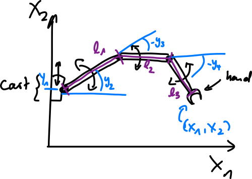
• e.g. inverse kinematics – consider 2D robot arm with 4 DOF
  • information loss when doing the forward kinematics (4D to 2D)
  • the simulation $X = \phi(Y)$ is defined as follows:
    • $X_1 = 0 + l_1 \cos(Y_2) + l_2 \cos(Y_2 + Y_3) + l_3\cos(Y_2 + Y_3 + Y_4)$
    • $X_2 = Y_1 + l_1 \sin(Y_2) + l_2 \sin(Y_2 + Y_3) + l_3\sin(Y_2 + Y_3 + Y_4)$
  • priors (“preferred joint positions”, “convenient situations”)
    • $p^S(Y) = p_1^S(Y_1) p_2^S(Y_2) p_3^S(Y_3) p_4^S(Y_4)$ independent
    • $p_1(Y_1) = \mathcal{N}(0, \sigma^2=\frac{1}{16})$
    • $p_{2,3,4}(Y_{2,3,4}) = \mathcal{N}(0, \sigma^2=\frac{1}{4})$ (radians)
  • given desired hand location $X^{\text{obs}}$, compute $p(Y \mid X^{\text{obs}}) \approx p^S(Y \mid X^{\text{obs}})$
  • $p^S(Y \mid X^{\text{obs}}) > 0$ for all $Y \in \mathcal{F}(X^{\text{obs}}) = \underbrace{\left\{Y \mid \phi(Y) = X^{\text{obs}}\right\}}_{\text{infinite since}\ \mathrm{dim}(Y) > \mathrm{dim}(X)}$
  • $p^S(Y \mid X^{\text{obs}}) \approx 0$ if $Y$ is inconvenient according to prior
  • $p^S(Y \mid X^{\text{obs}}) \gg 0$ if $Y$ is convenient according to prior
  • joint probability $p^S(X, Y) \propto \delta(X - \phi(Y)) \cdot p^S(Y)$

Validation of generative models (especially SBI)

• fundamental problem: if $X \sim p(X)$, there is no single correct outcome
  • $\Rightarrow$ traditional testing $\hat X_i = X^*_i$ doesn’t work
  • $\Rightarrow$ must compare distributions, no individual outcomes
    1. case: for prior, we have $\left\{X_i^* \sim p^*(X)\right\}_{i=1}^N$ for fixed $Y$
  • easily generated by simulation
    1. case: for posterior, we have $p(Y \mid X) \approx p^*(Y \mid X)$
  • to generate $\left\{Y_i \sim p^*(Y \mid X)\right\}_{i=1}^N$ for fixed $X^{\text{obs}}$, we need a classical algorithm (like MCMC or ABC)
• we can compare means/covariances of ${\hat X_i}$ and $\left\{X_i^*\right\}$ – quick check, complete if $p$ is Gauss
  • can also compare higher order momentums but this tends to be expensive
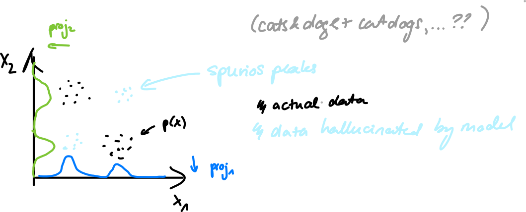
• plot marginal distributions in 1D and 2D for features $j, j' = 1, \ldots, D$
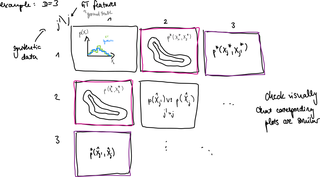
  • we don’t see correlations for higher dimensions but errors here can already be apparent
• various scores to compare the samples $\left\{\hat X_i\right\}_{i=1}^N$ and $\left\{X_i^*\right\}_{i=1}^N$ (usually $N=N'$):
  • (we already saw) MMD
  • Fredechet Inception Distance (FID) – popular if $X$ is an image
    • idea: compare means and covariance matrices via Fredechet distance
    • if they are Gaussian, the Fredechet distance (otherwise complicated) can be computed analytically as FD = ||\hat \mu - \hat^||^2 + \mathrm{tr}\left[\hat\Sigma - \Sigma^ - 2\left(\hat \Sigma \Sigma^*\right)^{1/2}\right]
    • for images Gaussian assumption is not fulfilled $\Rightarrow$ calculate FD in some feature space $h(X)$
      • typically, use a pre-trained network (traditionally Inception network, nowadays some foundational model eg. CLIP or DINOv2)
      • if no pre-trained model available, we can still use a random(ly initialized) network
  • density & coverage (heuristic version of MMD?) [Naeem et al 2020]
    • use nearest neighbor method, usually applied in a feature space to make Euclidean distance plausible
    • define $B_n(X_i)$ ball with center $X_i$ and radius $||X_i - X_{i_k}||_2$ for $i$ of the $k$-th nearest neighbour of $X_i$
      • $\Rightarrow \mathbf{1}\left[X' \in B_k(X_i)\right]$ is a kernel (the relation to MMD)
      • density = $\frac{1}{kN'} \sum_{i'=1}^{N'} \sum_{i=1}^{N} \mathbf{1}\left[\hat X_{i'} \in B_k(X_i^*)\right]$
        • high when the $\hat X_i$ are close to the $X_i^*$
        • $\mathbb{E}[\text{density}] = 1$ if all synthetic data is covered
      • coverage = $\frac{1}{N} \sum_{i'=1}^{N'} \mathrm{1}\left[\exists i\ \text{such that}\ \hat X_i \in B_k(X_{i'}^*)\right]$
        • counts how many of the balls around $X_i^*$ contain a $\hat X_i$
        • $\mathbb{E}[\text{coverage}] = 1 - \frac{1}{2^{k}}$ if the synthesized data nicely covers the real data
          1. case but we also don’t have $\left\{X_i^*\right\}_{i=1}^N$
  • $\Rightarrow$ must evaluate on the basis of $\left\{\hat X_i\right\}_{i=1}^N$ only, possibly with a single instance $X^* \sim p(X^*)$
    • e.g. grayscale coloring – we only have one GT image that we created the grayscale one from
  • check the diversity of the generated sample (always possible without any GT)
    • by diversity, we mean that $\left\{\hat X_i\right\}_{i=1}^N$ are all different and ideally cover the entire $p^*(X)$
    • Vendi score [Friedman & Dieng 2023]
      1. calculate kernel (Gram) matrix $G$:
         • $G_{i, i'} = \frac{1}{N} k(\hat X_i, \hat X_{i'})$ (can also be done in a feature space)
         • (missing in the paper) centralize $G$ as in kernel PCA (see MLE)
      2. calculate eigenvalues $\lambda_i$ of $G$
      3. calculate eigenvalue entropy $H(G) -\sum_{i} \lambda_i \log -\lambda_i$ (with $0 - \log 0 = 0$)
      4. $VS = \exp(H(G)) \le N$
      5. profit?
         • acts as an effective rank of $G$
         • if all points are far from each other: $G_{i, i'} \approx 0$ for $i \neq i'$ and $VS = N$ (max diversity)
         • if all points are equal, $G_{i, i'} = \frac{1}{N}$, we only have one non-zero eigenvalue and $VS = 1$
         • choosing kernel bandwidth correctly is critical to avoid the extreme cases

Validation of SBI

• given $\{\hat X_i \sim p(X)\}_{i=1}^N$ and $\{ X_i^* \sim p^*(X)\}_{i=1}^{N'}$
  1. case: $N' \approx N \gg 1 \Rightarrow$ compare the distribution of samples via methods from last lecture (MMD, FID, density/coverage)
  2. case: $N' = 0 \Rightarrow$ compare diversity of different approximations via Vendi score
  3. case: $N' = 1 \Rightarrow$ important case in practice
  • in SBI, create GT via forward simulation, $\left\{Y_i \sim p^S(Y), X_i \neq \Theta(Y_i, \varepsilon)\right\}$
    • $\Rightarrow Y_i$ is a GT example for $p(Y \mid X = \underbrace{X_i}_{\text{fixed}})$ with $N' = 1$
  • weather forecast: $p(Y = \text{rain tomorrow} \mid X = \text{weather up to now})$
    • $80\%$ rain probability – we can check how well it worked tomorrow
    • $Y_i = p^*(Y = \text{rain} \mid X = \text{weather so far})\ \hat =\ \text{actual weather}$
  • idea: “calibration” – merge instances with same predicted confidence in a joint test set
    • among all days with $80\%$ rain prob. it should have rained in $80\%$ of the cases
    • assumes that this is a reasonable thing to do (what if climate change?)
  • applied to classification: $p(Y=k \mid X)$ is $80\%$ and it answers right…
    • $80\%$ of the time – well calibrated
    • $>80\%$ of the time – underconfident
    • $<80\%$ of the time – overconfident
  • realization:
    • merge $$\underbrace{\left\{\hat Y_i \sim p(Y \mid X = \text{fixed})\right\}_{i=1}^{M}}_{\text{generated}} \lor \underbrace{\left\{Y_0 = Y^* \sim p^*(Y \mid X)\right\}}_{\text{GT}}$$
    • sort the merged set as $\left(Y_{[0]}, \ldots, Y_{[M]}\right)$ – GT should be uniformly placed
    • algorithm:
      1. given GT $Y^*$, sample $\left\{Y_k \sim p(Y)\right\}_{k=1}^N$
      2. sort the joined set $\left(Y_{i[0]}, \ldots, Y_{i[M]}\right)$
      3. $C = \frac{[k]}{M}$ (for $k$ index of $Y^*$ in sorted order)
         • repeat this for many $GT$ instances $X_i, Y_i \Rightarrow \left\{C_i\right\}_{i=1}^M$
      4. evaluate $\left\{C_i\right\}$ (it should be uniform) via histogram – if model is calibrated, $C_i \sim \mathrm{Binomial}(N, p=\frac{1}{2})$
         • TODO: graphs of what can happen – skewed - mean is wrong / canyon - overc. / valley – underc.
    • caveat: well-calibrated does not imply accurate
      • if the model is bad and it knows it, it’s still calibrated
      • example: $t$ time, sample mean on day $t$ $\mu_t \sim \mathcal{N}(0, 1), Y_t \sim \mathcal{N}(\mu_t, 1)$
        • marginal is $Y_t \sim p^*(Y_t) \sim \mathcal{N}(0, \sigma^2=2)$
        • TODO: finish this, it’s weird
      • the lecture has an alternative solution via empirical CDF of $C$s
        • we don’t have a hyperparameter (calculated automatically), which is useful
  • joint calibration checks: instead of using $\left(Y_{i[0]}, \ldots, Y_{i[M]}\right)$ on one feature at a time, check the entire vector
    • $\Rightarrow$ reduce the problem to 1-D via “energy” or “surprisal” distribution
    • probably TODO here since I got really lost; there should be an algorithm here

There is a missing lecture here! See slides for what was in it.

Epidemology: SIR model

• an example of SBI
• [Kermach & McKendrick 1927]
• Susceptible $S$: people who are healthy but can get infected
• Infected $I$: people who are ill and can transmit
• Recovered $R$: people who recovered and are now immune
• simplifying assumptions:
  • stationary dynamics: behavior of virus/bacteria and people does not change over time
    • no mutations, no countermeasures
  • only consider averages over all people in each compartment ($S$, $I$, $R$)
    • all people in the same compartment are considered identical
• traditional non-probabilistic parameter fitting: least squares $$\hat Y = \argmin_Y \mathbb{E}_{\eta \sim p^S(\eta)} \left[||X^{\text{obs}} - \Theta (Y, \eta)||^2\right]$$
  • $+$ makes the simulation reproduce the real observations as closely as possible
  • $-$ might get stuck in bad local optima (if the simulation isn’t linear with Gaussian noise)
  • $-$ disregards uncertainty and ambiguity in $Y$
• amortized SBI learns a GNN for $p(Y \mid X^{\text{obs}}) \approx p^S(Y \mid X^{\text{obs}})$
  • using a large $TS$ of synthetic data ($M=10\ 000+$)
• design model:
  • a healthy individual meets on average $\lambda_1$ people per day
  • infected people are not isolated, but meet others as usual
    • $\Rightarrow$ a fraction $I/N$ of the $\lambda_1$ meetings is potentially contagious
  • a fraction $\lambda_2$ of all the dangerous meetings actually leads to transmissions
  • if we observe a reduction in infections, we cannot distinguish if people became more cautious ($\lambda_1$ goes down) or the virus is less infections ($\lambda_2$ goes down)
    • $\Rightarrow$ can only recover $\lambda = \lambda_1 \lambda_2$
  • nobody dies and infected people recover after $\delta$ days
  • the rates are the following:
    • number of new infections per day: $\lambda \frac{I}{N} \cdot S$
    • number of recoveries per day: $\frac{1}{\delta} I = \mu I$ (for $\mu$ recovery rate)
  • write the dynamics as a system of ordinary differential equations – each line is the change in the compartment: $$\begin{aligned} \frac{dS(t)}{dt} = -\lambda \frac{I(t)}{N} S(t) \\ \frac{dI(t)}{dt} = \lambda \frac{I(t)}{N} S(t) - \mu I(t) \\ \frac{dR(t)}{dt} = \mu I(t) \end{aligned}$$
  • can divide all equations by $N$, getting normalized values: $$\begin{aligned} \frac{d[S(t)]}{dt} = -\lambda [I(t)] [S(t)] \\ \frac{d[I(t)]}{dt} = \lambda [I(t)] [S(t)] - \mu [I(t)] \\ \frac{d[R(t)]}{dt} = \mu [I(t)] \end{aligned}$$
  • to solve equations, must define $t=0$:
    • $I_0 = [I(t=0)] = \mathrm{const}$
    • $R_0 = [R(t=0)] = 0$
    • $S_0 = [S(t=0)] = 1 - I_0$
  • given $I_0, \lambda, \mu$, we can solve the ODEs for any time by “integration”
    • Euler forward method: discrete timesteps $\Delta t$, approximate
      • $[S(t + \Delta t)] = [S(t)] - \lambda [I(t)] [S(t)] \cdot \Delta t$
      • same for other equations…
      • theory says that it’s a good approximation if $\Delta t$ is small enough
    • more sophisticated: Euler backward, Runge-Hutta that allow for larger timesteps
  • define observables $X$:
    • repeat on every day (number of new infections and newly recovered)
    • observations are not perfect $\Rightarrow$ observation model
      • reporting $\Delta S^{\text{obs}}(T) = f(\Delta S^*(t - L))$ for $L$ delay
      • underreporting: $\Delta S^{\text{obs}} \sim S \Delta S^*$
      • there is some noise going on
    • exact values:
      • $\Delta S^*(t) = S^*(t - \Delta t) - S^*(t)$
      • $\Delta R^*(t) = R^*(t) - R^*(t - \Delta t)$
    • measured values:
      • $\Delta \tilde S (t) = \Delta S^* (t - L) \cdot \varepsilon_S \quad S \sim \mathcal{N}\left(S, \sigma^2\right)$
        • we get relative error, because we’re multiplying
      • same for others (noise can be same / different)
    • full simulation: $Y = \left[I_0, \lambda, \mu, L, S, \sigma^2\right] \sim p^S(Y)$
      • usually $p^S(Y) = p^S(I_0)p^S(\lambda)p^S(\mu)p^S(L)p^S(S)p^S(\sigma^2)$
      • should be chosen according to epidemiological prior knowledge
    • $X = \Theta(Y, \eta)$
      • TODO: equations for the simulation
      • get the true values from ODE, calculate noise from the observables (diff between truth and what we can measure)
      • we can’t observe the actual state (ODES) but only the noise
    • full algorithm:
      1. define the simulation $\Theta(Y, \eta)$ and priors $p^S(Y)$ and $p^S(\eta)$
      2. use the simulation to generate synthetic TS
      3. setup architecture of GNN
         • TODO: image here
      4. train SNF & summary network jointly using NLL loss: $$\hat p, \hat h = \argmin_{p, h} \frac{1}{M} \sum_{i=1}^{M} -\log p(Y_i \mid h(X_i))$$
         • $h(X)$ will become optimally informative for $p(Y \mid h(X))$
      5. validate $\hat p, \hat h$ (check calibration, sensitivity, etc.)
         • tells us that it models the synthetic data well, not the real data
      6. infer $\hat p(Y \mid h(X^{\text{obs}}))$ for real data
      7. check for potential simulation gap ($\hat =$ simulation is unrealistic)

New lecture here, we’re doing SBI for epidemiology again.

• a typical person will on average transmit to $$\delta \lambda \cdot \overline{[S(t)]}$$ healthy people (duration times change of infection times average number of healthy people the person meets in those days)
• basic reproduction number is $$R_0(t) = \delta \lambda(t) \begin{cases} >1 & \text{new infections go up} \\ <1 & \text{new infections go down} \end{cases}$$ (here $\lambda$ is a function of $t$ if there are eventually countermeasures / disease mutations)
• replacement number $$r(t) = R_0(t) [S(t)] \begin{cases} >1 & I(t)\ \text{grows} \\ <1 & I(t)\ \text{shrinks} \end{cases}$$
• $\Rightarrow$ two possibilities to end disease:
  1. herd immunity – when $r(t) < 1 \iff [S(t)] < R_0(t)$
  2. by countermeasures – reduce $\lambda(t)$ s.t. $r(t) < 1$ (regardless of $S$)
• if $\lambda(t)$ changes over time, learning identification problem becomes much harder
• for a simulation to be realistic, implementing the fundamental mechanistic equations is not enough – a realistic model of observation uncertainty is required
  • (use squared loss in traditional inverse inference $\iff$ assumes additive Gaussian noise with constant variance)
  • model reporting delays

Making things more complex (because we can)

• new things:
  • deadly disease – introduce new compartment $D$ (dead) with new variable $\alpha$ for how many die
  • immunity lost after a while – transitions $R \rightarrow S$
  • vaccination – transition $S \rightarrow R$
  • imperfect immunity – new compartment $V$ (like $S$ but with $\lambda_V < \lambda_S$)
• refine infection:
  • incubation period (carrier) – infected but cannot transmit
    • $S \rightarrow C \rightarrow I$ (with new variable $\kappa$ for when they can transmit)
  • some (many) infections are undetected
    • split $I$ into “treated” (knows its infected) and “spreader” (can transmit without knowing it)
• further refinements:
  • split into risk groups (e.g. by age, sex, etc.)
  • spatial relations (hot spots, travel)
    • spatial compartments
      • discrete – every node becomes an SIR model, edges are spatial transmissions
      • continuous – PDE (partial differential equations)
  • $\lambda(t), \mu(t)$ change over time based on a lot of factors

Checking if the simulation is realistic

• different to calibration – here we have outside data (as opposed to the internal validation where we have our own data)
• Is $X^{\mathrm{obs}}$ (real observation or from a competing theory) covered by our SBI model?
  • yes $\rightarrow$ $p(Y \mid X^{\mathrm{obs}})$ can be trusted (if our model is well calibrated etc.)

Idea: if $X^{\mathrm{obs}}$ is an outlier of the marginal then networks have not seen data like it during training:

1. learn a surrogate for $p(X) \approx p^S(X)$ (expensive, big neural network)
2. get outlier detection almost for free: we have a summary network $h(X)$

Continuing with new lecture here.

Model misspecification detection: is $x^{\mathrm{obs}}$ an outlier?

• if yes, reject and answer “idk” 🤷
• trick: exploit the feature detection network: add loss $\kappa \mathrm{MMD}(p(h(X)) \mid \mathbb{N}(0, \mathbb{I}))$ to pull summary feature distribution towards standard normal
• reject $X^{\mathrm{obs}}$ if $h(X^{\mathrm{obs}})$ is an outlier of $\mathbb{N}(0, \mathbb{I})$

Model comparison & selection (between competing theories): measuring training error might not be enough because of overfitting.

• need tradeoff between model accuracy and complexity (“Occam’s razor”)
  • classical model selection criterion:
    • Akaika criterion $\mathrm{AIC} = 2 \mathbb{E}[NLL] + 2 \cdot \text{size}$ (for the size of the model)
      • if both models are equally good but one is smaller, it wins
    • Bayesian information criterion: $\mathrm{BIC} = 2 \mathbb{E}[NLL] + \log(N)$ (for $N$ dataset size)

Some more stuff was here but brain small.

External validation algorithm:

• given competing theories $\mathcal{M}_1, \ldots, \mathcal{M}_L$
  • epidemiology: different compartments, priors, observation uncertainty etc.
    1. create synthetic training data $$TS_l = \left\{\left(Y_{il} \sim p(Y \mid \mathcal{M} = l), X_i \sim p(X \mid Y_{ill}, \mathcal{M} = l)\right)\right\}_{i=1}^{N_l}$$
    2. train a separate SBI model for each $TS_l$ with $\text{MMD}$ so that $p(h_l(X)) = \mathcal{N}(0, \mathbb{I})$
    3. perform internal validation for each $l$, redesign $\text{SBI}_l$ until successful
    4. train a sofmax classifier $p(\mathcal{M} \mid X)$ using combined $\mathrm{TS}$
  • $\hat p(\mathcal{M} \mid X) = \argmin_P \frac{1}{L} \sum_{l=1}^{L} \frac{1}{N_l} \sum_{i=1}^{N_l} -\log p(\mathcal{M} = l \mid X = X_{il})$
    1. external validation given $X^{\text{obs}}$
  • model misspecification detection
  • compute logits of model classifier $S_l$ (penultimate layer, before sofmax)
  • define classifier $p(\mathcal{M} \mid X^{\text{obs}}) = \mathrm{softmax}(S_l: l \in \mathcal{M}^{\mathrm{in}})$
  • model comparison by posterior odds

Parameter degeneracy

• sometimes, some elements in $Y$ cannot be fully identified from $X$
  • correlations in the posteriors
• example: epidemiologist write SIR equations in terms of natural/conceptual parameters
  • $\lambda_1$: average number of people a healthy person meets per day
  • $\lambda_2$: fraction of meetings leading to transmission
  • in SIR equatoins, we always have $\lambda_1 \lambda_2 \implies$ cannot distinguish them, but can infer $\lambda = \lambda_1 \lambda_2$
  • if we still use $\lambda_1, \lambda_2 \implies$ posterior shows the degeneracy (infinitely many pairs ($\lambda_1, \lambda_2$) for fixed $\lambda = \lambda_1 \lambda_2$)
  • degeneracy is easy to spot, but generally difficult and hard to distinguish from bad convergence of neural network

Lecture talks about SoftFlow here which addresses this issue for cNFs.

• do not confuse with NoiseNet, which adds the noise to $X$ (here we add to $Y$)

This lecture had slides with some interesting use cases of the methods that we previously discussed.

Hierarchical models for SBI

• split hidden parameters into $Y = [Y^G, Y^I]$
  • $Y^G$ – global (for the entire population)
  • $Y^I$ – individual (for every instance)
• example – virology:
  • $Y^G$ – properties of a patient (& disease)
  • $Y^I$ – properties of individual cells we analyse
• simulation:
  • $Y^G \sim p^S(Y^G)$ (standard SBI)
  • $Y^I \sim p^S(Y^I \mid Y^G)$ (for every individual)
  • $X_i = \Theta(Y^G, Y^I_i, \eta_i)$ for $\eta_i \sim p^S(\eta)$
    • common simplification is $\Theta(Y^I_i, \eta_i)$

Here we discuss Estimation of a non-linear mixed effects model [Arruda et al 2023].

SINDy-Autoencoders

• “Sparse Identificator of Non-Linear Dynamics”
• we have a dynamic system that produces real-world measurements
• observation takes place in a different coordinate system (e.g. measurements of the planets from earth’s perspective/unknown canonical coordinates)

Two lectures were spent on this.

Physics-informed Neural Networks (PINNs)

• idea: use physical prior knowledge explicitly
  • (so far SIB knowledge only used to create training set)
  • PINNs: incorporate knowledge into training
• PINNs focus on surrogates for forward problem
  • reminder: SBI – $X = \Phi(Y, \eta), Y \sim p(Y), \eta \sim p(\eta) \iff p(X \mid Y) p(Y)$
    • surrogates learn the likelihood (what we focus on now)
    • SBI usually learns posterior of inverse problem ($p(Y \mid X)$)
• typically, PINNs only give a single solution, not a distribution
  • i.e. learn $\Phi(Y, \eta)$ for $Y$ and $\eta$ fixed (known or learned)
• PINNs address the case where $X$ is a function
  • this is the case in physics – real world is a function, not a vector
  • surrogate $\hat\Phi(\vec u, t; Y, \eta)$ (for $t$ time and $\vec u$ space, which can be present)
  • $\Phi(t)$ is a solution of ODE, $\Phi(\vec u t, Y, \eta)$ is a solution of PDE
• physical prior knowledge: formula for the ODE or PDE

Why is this useful?

• actual simulation may be too expensive (e.g. Schrödinger)
• requires a lot less training data than traditional SBI

Example: growth data (real, not simulated)

TODO: image here

• idea: use physical knowledge as a problem-specific regularizer
• here the growth follows the “logistic rule”: $\frac{\partial f(t)}{\partial t} = \lambda f(t) (1 - f(t))$
  • we may or may not know $\lambda$ (depending on the problem)
  • special case of SIR equations – the lecture has a derivation here
• PINN approach to learning:
  • two bounds of points (later 3)
    • data points $\hat =$ TS where $f(t)$ is (approximately) known (at least the data for initial condition)
    • collocatoin points where we apply the regularizer
      • $t \in \mathrm{CP}$: check if ODE is fulfilled at $t$
  • regularization term: $$\mathrm{loss}_{\mathrm{ODE}} = \frac{1}{M} \sum_{m=1}^{M} \left(\frac{\partial f(t_m)}{\partial t} - \lambda f(t_m)(1-f(t_m))\right)^2$$
    • if fulfilled then it should be zero for any $t_m$ (ideally $M \mapsto \infty$)
  • data term: $$\mathrm{loss}_{\mathrm{data}} = \frac{1}{N} \sum_{i=1}^{N} \left(f_i - f(t_i)\right)^2$$

The regression problem is now just $$\hat f, \hat \lambda = \argmin_{f, \lambda} \nu_{\mathrm{data}} \mathrm{loss}_{\mathrm{data}} + \nu_{\mathrm{ODE}} \mathrm{loss}_{\mathrm{ODE}}$$

• we do not get a distribution over functions $p(f(t) \mid \mathrm{data})$

The lecture talks here about the general case for ODEs.

Benefits of using NNs:

• universal approximators (if big enough) and good convergence in practice
  • $\Rightarrow$ can in practice learn any $f^*(t, Y)$
• derivatives $f(t) \dot f(t), \ddot f(t)$ easily computable by autodiff

Disadvantages of using NNs:

• for each set of data points and parameters, training must be restarted (no amortization)
  • problem is currently addressed (later

Tips and tricks:

• use $\tanh(u)$ activation or recently $\mathrm{GELU}$
• standardize the problem (similar to sclaing features to unit variance)
  • translate ODE into a “dimensionless” form (use fractions instead of absolutes)
    • nice constraint for $0 \le f(t) \le 1$
• random Fourier features – convert features into the Fourier domain with random projections
  • was shown that low-frequency behavior converges much faster than high-frequency
• random weight factorization (replace a linear layer with I don’t know)

PINN-related things (training, variants).

State-of-the-art generative modeling

• our current workhorse are invertible neural networks (affine or spline coupling flows)
• the directions of improvement:
  1. lift architectural restrictions that only facilitate efficient training
     • free-form flows
       • potentially higher expressive power (very new)
       • opportunity to incorporate application-related architecture restrictions
       • allows for bottleneck architectures
  2. get higher fidelity of the generated data (image generation, molecular modeling)
     • diffusion models
       • can generate better data but can’t generate the probability well
  3. speed-up generation and inference
     • consistency models & injective flows

Free-form flows

• [Draxler, Sorrenson et al. 2023]
• use arbitrary (dimension-preserving) neural networks as encoder and decoder
  • e.g. variations of ResNet
• give up invertibility of encoder: $g(z) = f^{-1}(z)$ by construction
  • instead train two separate networks and ensure $g(z) \approx f^{-1}(z)$
  • $\Rightarrow$ reconstruction loss $\mathcal{l}_{\mathrm{rec}} = \mathbb{E}_{x \sim p^*(\lambda)} \left[||x - g(f(x))||^2_2\right]$
• train generative distribution by the maximum likelihood
• express $p(x)$ with the change of variables formula p(x) = g(z=f(x)) \left|\det \frac{\partial f(x)}{\partial x}\right| \approx g(z=f(x)) \left \det \frac{\partial g(z=f(x))}{\partial z}\right^{-1}
• coupling flows exist to make $\left| \det \frac{\partial f(x)}{\partial x} \right|$ tractable
• two types of layers in coupling flows
  • rotation / permutation layers: $z^{(l)} = Qz^{(l-1)}$ for $Q$ orthonormal
    • $\frac{\partial z^{(l)}}{\partial z^{(l-1)}} = Q \implies \left|\det \frac{\partial z^{(l)}}{\partial z^{(l-1)}} = 1\right|$
  • coupling layers (generally auto-regressive blocks)
    • $\frac{\partial z^{(l)}}{\partial z^{(l-1)}} = \mathcal{J}^{(l)}$ is triangular $\implies \left|\det \frac{\partial z^{(l)}}{\partial z^{(l-1)}} = \prod_{j=1}^{D} \mathcal{J}^(l)_{jj}\right|$
• if layer architecture is free, these tricks no longer work $\implies$ must calculate $\frac{\partial f(x)}{\partial x}$ by autodiff
  • modern autodiff can do this reasonably but for $D \in \mathcal{O}\left(10^2 \ldots 10^3\right)$
  • autodiff offers library functions for Jacobian-vector products (jvp) and vector-Jacobian products (vjp)
    • can use without actually explicitly constructing the Jacobian
  • if $v$ is a unit vector, we get a column of $\frac{\partial f}{\partial x}$
    • $\Rightarrow$ construct $\frac{\partial f}{\partial x}$ explicitly by $D$ jvp products
  • fast enough for inference but slow during training – to make it efficient, you do not need $\left|\det \frac{\partial f}{\partial x}\right|$ – for training, we only need $\nabla{\Theta} \log \left|\det \frac{\partial f_{\Theta}}{\partial x}\right|$ with network parameters $\Theta$
    • surprising result: this can be estimated efficiently without access to $\frac{\partial f}{\partial x}$

The lecture shows the derivation for why this is the case here.

$\boxed{\nabla\Theta \mathcal{l}_{\mathrm{NLL}} \approx \mathbb{E}_{x \sim p(x)} \left| \nabla\Theta - \log g(z=f_\Theta(x)) - \nabla_\Theta \left(\text{stop-gradient}\left(\text{vjp}(g_\Theta, z=f_\Theta(x), v)\right) \cdot \text{jvp}(f, x, v)\right) \right|}$ $$\mathcal{l}_{\mathrm{total}} = \mathcal{l}_{\mathrm{NLL}} + \beta \mathcal{l}_{\mathrm{rec}}$$

• experiments:
  • FFF works as well as other NFs on toy data
  • FFF works very well on simple molecular modelling benchmarks

Injective flows

• NF with a bottleneck: $\dim(z) < \dim(x)$

Fever dream.

Bottleneck Free-form Flows

• $g(z) = z \cdot v$ is linear
  • consistency requirement: $z = f(g(z))$
  • we get $f(z \cdot v) = z\quad f(\alpha \cdot z v) = \alpha z \implies f(x)$ is also linear $v = \begin{bmatrix} a \\ c \end{bmatrix}, w^T = \begin{bmatrix} b & d \end{bmatrix} \implies w^T v z = z \implies d = \frac{1 - ab}{c}$
  • infinitely many solutions for $w^T$ if $v$ is fixed
• $g(z) = z v + t \implies f(x) = w^T(x - t)$ – even worse
  • for non-linear pseudo-inverse pairs $f(x), g(z)$, ambiguity is even worse
  • open problem for higher dimensions

We can formalize the quesiton:

• encoder defines equivalence classes of data points $x$ mapped to the same code $z$ $$\mathcal{F}(z) = \left\{x \mid f(x) = z\right\}$$
• decoder defines a representative $\hat x = g(z)$ for each fiber $$\mathcal{M} = \left\{\hat x = g(z) \mid z \in \mathcal{Z}\right\}$$
• with two constraints:
  1. $\hat x = g(z) \in \mathcal{F}(z)$, s othat $f(g(z)) = z$
  2. if $g(z)$ is continuous, $\mathcal{M}$ is also continuous
• even if $f(x)$ (and $\mathcal{F}(z)$) are fixed, infinitely many $\mathcal{M}$ are still possible
  • same goes for $\mathcal{M}$
• how to train an injective free-form flow?
  • to use NLL loss, we need a change-of-variables formula
  • rectangular/injective c-o-v formula for decoder p(\hat x = g(z)) = g(z) \cdot \left| \det\left(\underbrace{\left(\frac{\patial g}{\partial z}\right)\cdot \left(\frac{\partial g}{\partial z}\right)^T\right)}_{d\times D \cdot D \times d}\right|^{- \frac{1}{2}}
    • this is a probability on $\mathcal{M}$; says nothing about $x \in \mathcal{M}$
• need to learn three things:
  1. manifold $\mathcal{M}$ that represents well under lossy compression
  2. fibers $\mathcal{F}(z)$ which differences between $x$ and $x'$ we choose to ignore
  3. $p(\hat x)$ as distribution of points after projection $g(f(x))$
• much more difficult than NF, which only learn $p(x)$
• the squared reconstruction loss $$\mathbb{E}_{x \sim p^x(x)} \left[||x - g(f(x))||^2_2\right]$$ gives reasonable $\mathcal{M}$ and $\mathcal{F}(z)$ in practice
  • $\mathcal{M}$is a kind of average of the original $\mathrm{TS}$ (in lower dimension)
  • $\mathcal{F}(z)$ tend to be orthogonal to $\mathcal{M}$(in Euclidean norm)
• $\Nabla_\Theta \mathcal{L}_{\mathrm{NLL}}$ can be computed by an adapted version of FFF
  • training only with $\mathcal{L}_{\mathrm{NLL}}$ (as in standard NF) is impossible (leads to degenerate solutions)

Results: injective FFFs are competitive on standard benchmarks

• scaling it up to serious applications is an open problem

FFFs for data on a known manifold $\mathcal{M}$ (don’t have to learn it)

• further assume that the projection function $\hat x = \mathrm{proj}(x)$ is already known
  • $\Rightarrow$ we also don’t have to learn $\mathcal{F}(z)$
• e.g. data are on the surface of the earth (manifold is sphere, projection is orthogonal)
  • define $g(z)$ only on $\mathcal{M}$, not on $\mathcal{X} \implies g(z)$ already has correct topology
  • if $\mathcal{M}$ has finite volume (earth surface area), $g(z) = \mathrm{uniform}(\mathcal{M})$ is a good choice
• trick: train proto-encoder $\tilde f_{\Theta} (x \in \mathcal{M}) \mapsto \mathcal{X}$ and proto-decoders $\tilde g_{\Theta}(z \in \mathcal{M}) \mapsto \mathcal{X}$
  • higher expressive power by exploiting large space $\mathcal{X}$ instead of restricting to $\mathcal{M}$
• actual encoder and decoder are defined by projection:
  • $f_\Theta(x' \in \mathcal{M}) = \mathrm{proj}\left(\tilde f_\Theta\left(x \in \mathcal{M}\right)\right) \in \mathcal{M}$
  • $g_\Theta(z' \in \mathcal{M}) = \mathrm{proj}\left(\tilde g_\Theta\left(z \in \mathcal{M}\right)\right) \in \mathcal{M}$

TODO image here

• the FFF trick still works (with a minor modification)
• benefits
  • $+$ simpler than most competing methods on manifolds
  • $+$ can be trained by NLL loss
  • $+$ quite good results on simple benchmarks
• drawbacks
  • $-$ not quite state of the art
  • $-$ not tested on real problems