slama.dev

Introduction to Machine Learning

notes · 21. 4. 2023 · [edit]

• Resources
• Introduction
• Notation
  • Types of learning approaches
• Classification
  • Deterministic classifier
  • Probabilistic classifier
  • Threshold classifier
  • Bayes rule of conditional probability
    • How good can it be?
    • How bad can it be?
  • Linear classification
    • Perceptron
    • Rosenblatt’s algorithm
    • Support Vector Machine (SVM)
    • Linear Discriminant Analysis (LDA)
    • Logistic regression (LR)
    • Summary
    • Multi-class classification
  • Non-linear classification
• Neural networks
  • Convolutional Neural Networks (CNNs)
  • Receptive field of a neuron
  • Some history
  • Residual Networks (ResNet)
  • Training
    • Data augmentation
    • Self-supervised training
  • U-Net
• Regression
  • Linear regression
    • LSQR
    • Least Squares v2.0
  • Alternating optimization
  • Regularized regression
    • Ridge regression
    • Bias-variance trade-off
    • Other regularization terms
  • Non-linear regression
    • Decision trees / forests

Preface

This website contains my lecture notes from a lecture by Ullrich Köthe from the academic year 2022/2023 (University of Heidelberg). If you find something incorrect/unclear, or would like to contribute, feel free to submit a pull request (or let me know via email).

The notes end at the decision tree/forest lecture (inclusive)!

Also, special thanks to Lucia Zhang, some of the notes are shamelessly stolen from her.

Resources

• TensorFlow playground – a really cool visualization of resigning and training a neural network for classification/regression and a number of standard parameters (activation functions, training rates, etc…)

Introduction

Setting:

• quantities $Y$ that we would like to know but can’t easily measure
• quantities $X$ that we can measure and are related to $Y$

Idea:

• learn a function $\hat{Y} = f(X)$ such that $\hat{Y}_i \approx Y_i^*$ (we’re close to the real value)

Traditional approach:

• ask an expert to figure out $f(X)$, but for many approaches ML works better

Machine learning:

• choose a universal function family $F$ with parameters $\theta$
  • ex. $F = \left\{ax^2 + b + c\right\}, \theta = \left\{a, b, c\right\}$
• find parameters $\hat{\theta}$ that fit the data, so $$\hat{Y} = f_{\hat{\theta}}(X) \qquad \text{and} \qquad \hat{Y}_i \approx Y_i^*$$

Basic ML workflow:

1. collect data in two datasets: training dataset (TS) to train and test dataset to validate
   • extremely important, if you don’t do this you die instantly
   • necessary for recognizing overfitting ($F$ is polynomials and we fit points…)
2. select function family $F$
   • prior knowledge about what the data looks like
   • trial and error (there are tools to help you with this)
3. find the best $\hat{\theta}$ by fitting $F$ to the training set
4. validate the quality of $f_{\hat{\theta}}(X)$ on the test set
5. deploy model in practice

Probabilistic prediction:

• reality is often more complicated
• no unique true response $Y^*$, instead set of possible values (possibly infinite)
• in that case we learn a conditional probability (instead of a function): $$\hat{Y} \sim p(Y \mid X)$$
• to learn this, we define a “universal probability family” with parameters $\theta$ and chose $\hat{\theta}$ such that $$Y \sim p_{\hat{\theta}}(Y \mid X)$$ matches the data
• strict generalization: deterministic case is recovered by defining $p(Y \mid X) = \delta(Y - f(X))$
  • $\delta$ distribution has only one value
• often we derive deterministic results from probabilistic predictions (eg. mode/median/random sample of the distribution)
  • generally, mode is the best, has some really nice properties

Problems:

• nature is not fully predictable
  • quantum physics (randomness)
  • deterministic chaos (pendulum)
  • combinatorial explosion (aminoacids)
• data:
  • finite
  • noisy
  • incomplete
  • ambiguous
• model:
  • function family is imperfect (too small)
  • may not have converged
  • nature has changed in the meantime
• goal:
  • disagreement about what is relevant (desirable)
• handling uncertainty is central challenge of AI and ML

Notation

• features vector $X_i$ for each instance $i \in 1, \ldots, N$
• feature matrix $X$ (rows are instances, columns are features $j \in 1, \ldots, D$)
  • $X \in \mathbb{R}^{N \times D}$

$i \setminus j$	$1$ (name)	$2$ (height)	$3$ (gender)
$1$	Alice	$1.7$m	f
$2$	Bob	$1.8$m	m
$3$	Max	$1.9$m	m

We usually (when Programming) want a float matrix: drop names, discretize labels and use one-hot encoding (one-hot because there is only ones in the particular features).

$i \setminus j$	$1$ (height)	$2$ (f)	$3$ (m)	$4$ (o)
$1$	$1.7$	$1$	$0$	$0$
$2$	$1.8$	$0$	$1$	$0$
$3$	$1.9$	$0$	$1$	$0$

• response $Y_i$ row vector for instance $i$, response elements $m \in 1, \ldots, M$
  • most of the time, $M = 1$ (scalar response)
  • exception is one-hot encoding of discrete labels
• tasks according to type of response
  • $Y_i \in \mathbb{R}^M \ldots$ $Y \approx f_\theta(X)$ is regression
  • $Y_i = k; k \in \left\{1, \ldots, C\right\}$ for $C$ number of categories $\ldots$ classification
    1. labels are ordered (“tiny” < “small” < “medium” < “large”) – ordinal classification
    2. labels are unordered (“apples”, “oranges”) – categorial classification
• training set $\mathrm{TS} = \left\{(X_i, Y_i)\right\}_{i = 1}^N$ – supervised learning
  • $Y_i$ is the known response for instance $i$

Types of learning approaches

1. supervised learning – true responses are known in $\mathrm{TS} = \left\{(X_i, Y_i)\right\}_{i = 1}^N$
2. weakly supervised learning
   1. we have some information (know $Y_i$ for some instances)
   2. we have worse information (there is a tumor but we don’t know where)
3. unsupervised learning – only features are known in $\mathrm{TS} = \left\{X_i\right\}_{i = 1}^N$
   • learning algorithm must find the structure in the data on its own (data mining or, for humans, “research”)
   • only a few solutions that are guaranteed to work (this is unsurprisingly difficult to do)
     1. representation learning – compute new features that are better to predict
     2. clustering – group similar instances into “clusters” with a single representative
4. self-supervised learning – define an auxiliary task where $Y_i$ are easy to determine

Classification

• $Y_i = k, k \in \left\{1, \ldots, C\right\}$
  • common special case $C = 2$, then $k \in \left\{0, 1\right\}$ or $k \in \left\{-1, 1\right\}$
• always supervised!

Deterministic classifier

• one hard prediction for each $i$ $$\hat{Y}_i = f(X_i) \quad \text{with} \quad \hat{Y}_i = Y_i^*$$

Quality measured by collecting the “confusion matrix”

$\hat{Y} \setminus Y^*$	$-1$	$+1$
$-1$	true negative	false negative
$+1$	false positive	true positive

1. false positive/negative fraction – “how many out of all events are false” $$\frac{\# \mathrm{FP}\ \text{or}\ \# \mathrm{FN}}{\mathrm{N}} \in \left[0, 1\right]$$
2. false positive/negative rate – “how many out of positive/negative events are false” $$\frac{\# \mathrm{FP}}{\# \mathrm{FP} + \# \mathrm{TN}} \approx p(\hat{Y} = 1 \mid Y^* = -1) \qquad \frac{\# \mathrm{FN}}{\# \mathrm{FN} + \# \mathrm{TP}} \approx p(\hat{Y} = -1 \mid Y^* = 1)$$

Probabilistic classifier

• returns a probabilistic vector $\in [0, 1]^C$ (soft response) for every label $\equiv$ posterior distribution $$p(Y = k \mid X)$$
• more general than hard classification – can recover decision function by returning the most probable label by using $\arg \max$: $$p(Y = k \mid X) \implies f(X) = \arg \max_k\ p(Y = k \mid X)$$

Quality measured by “calibration”

• if $p(Y = k \mid X) = v$, then label $k$ should be correct $v\%$ of the times
  • if actual accuracy is higher, then the classifier is “under confident”
  • otherwise it’s “over confident” (often happens)

Important: calculate confusion matrix or calibration from test set, not train set (bias)!

Threshold classifier

• single feature $X \in \mathbb{R}$
  • usually not enough to predict the response reasonably
• $\hat{Y} = \mathrm{sign}(X - T) = \begin{cases} 1 & X > T \\ -1 & X < T \end{cases} \quad$ for some threshold $T$
• three classical solutions for multiple features
  1. design a formula to combine features into single score (use BMI for obese/not obese)
     • hard and expensive for most problems, not to mention inaccurate
  2. linear classification: compute score as a linear combination and learn coefficients
     • $S_i = \sum_{j = 1}^{D} \beta_j X_{ij} \implies \hat{Y}_i = \mathrm{sign}(S_i - T)$
     • less powerful than the first one (restricted to linear formulas)
     • we can learn so it usually performs better
  3. nearest neighbour: classify test instance $X_{\text{test}}$ according to most similar training instance
     • $\hat{i} = \arg \min_i\ \mathrm{dist(X_i, X_{\text{test}})}$
     • then $\hat{Y}_{\text{test}} = Y^*_{\hat{i}}$
     • expensive – to store the entire training set and scan it for every $X_{\text{test}}$
       • doesn’t scale well for more features (generalized binary search)
     • hard to define the distance function to reflect true similarity
       • “metric learning” is a hard task of its own…

Bayes rule of conditional probability

• joint distribution of features and labels $p(X, Y)$
• can be decomposed by the chain rule to
  • $p(X) p(Y \mid X)$ – first measure features, then determine response
  • $p(Y) p(X \mid Y)$ – first determine response, then get compatible features
• for classification, we want to use Bayes rule $$\boxed{\underbrace{p(Y = k \mid X)}_{\text{posterior}} = \frac{ \overbrace{p(X \mid Y = k)}^{\text{likelihood}}\ \overbrace{p(Y = k)}^{\text{prior}} }{\underbrace{p(X)}_{\text{marginal}}}}$$
  • posterior – we want to update our judgement based on measuring the features
  • prior – we know this (1% for a disease in the general population)
  • likelihood – the likelihood of the disease given features (fever, cough)
  • marginal – can be recovered by summing over possibilities: $$p(X) = \sum_{k = 1}^{C} p(X \mid Y = k)$$

Is hugely important for a number of reasons:

• fundamental equation for probabilistic machine learning
  • allows clean uncertainty handling (among others)
• puts model accuracy into perspective (what is good or bad)
• defines two fundamental model types:
  • discriminative model: learns $p(Y = k \mid X)$ (right side)
    • answers the question “what class” directly
    • (+) relatively easy – take the direct route, no detour
    • (-) often hard to interpret how the model makes decisions (black box)
  • generative model: learns $p(Y = k)$ and $p(X \mid Y = k)$ (left side)
    • first learn how “the world” works, then use this to answer the question
      • $p(X \mid Y = k)$ – understand the mechanism how observations (“phenotypes”) arise from hidden properties
    • (-) pretty hard – need powerful models and a lot of data
    • (+) easily interpretable – we can know why it was answered
• ex.: breast cancer screening: $p(Y = 1) = 0.001, p(Y = -1) = 0.999$
  • a test answers the following
    • correct diagnosis: $p(X = 1 \mid Y = 1) = 0.99$
    • false positive: $p(X = 1 \mid Y = -1) = 0.01$
  • if the test is positive, should you panic? $$\begin{aligned} p(Y = 1 \mid X = 1) &= \frac{p(X = 1 \mid Y = 1) p(Y = 1)}{p(X)} \\ &= \frac{0.99 \cdot 0.001}{0.99 \cdot 0.001 + 0.01 \cdot 0.999} \\ &\approx \mathbf{0.1} \end{aligned}$$
    • due to the very low probability of the disease, you’re likely fine

Some history behind ML:

• traditional science seeks generative models (we can create synthetic data that are indistinguishable from real data)
  • physics understand the movement of an object, so a game can use this to appear real
• ~1930: ML researches realized that their models were too weak to do this $\implies$ field switched to discriminative models
• ~2012: neural networks solved many hard discriminative tasks $\implies$ the field is again interested in generative models (Midjourney, ChatGPT, etc.)
  • subfield “explainable/interpretable ML”

How good can it be?

Definition (Bayes classifier): uses Bayes rule (LHS or RHS) with true probabilities $p^*$

• we don’t know $p^*$, we want to get as close as possible

Theorem: no learned classifier using $\hat{p}$ can be better than the Bayes classifier.

• if our results are bad, we have to get better theory (more features)

How bad can it be?

• case 1: all classes are equally probable ($p(Y = k) = \frac{1}{C}$)
  • worst classifier: pure guessing – correct $50\%$ of the time
• case 2: unbalanced classes
  • worst classifier: always return the majority label

Linear classification

1. use a linear formula to reduce all features to scaled score
2. apply threshold classifier to score ($C = 2$ for now)

$$\hat{Y}_i = \mathrm{sign}\left(\sum_{j} \beta_j X_{ij} + b\right)$$ for feature weights $\beta$ and intercept $b$.

• learning means finding $\hat{\beta}$ and $\hat{b}$
• we can also get rid of $b$ by one of the following:
  1. if all classes are balanced ($p(Y = k) = \frac{1}{C}$) then we can centralize features $$\bar{X} = \frac{1}{N} \sum_{i = 1}^{N} X_i \qquad \overset{0}{X_i} = X_i - \bar{X}_i$$
  2. absorb $b$ into $X$: define new feature $X_{i0} = 1$ (will then act as $b$)
     • done quite often ($X_{i0}$ is then called the “bias neuron”)

Perceptron

• Rosenblatt, 1958
• first neural network (1 neuron)
• idea: improve $\beta$ when model makes mistakes
  • naive approach – 0/1 loss: $$\mathcal{L}(\hat{Y}_i, Y^*_i) = \begin{cases} 0 & \hat{Y}_i = Y^*_i \\ 1 & \hat{Y}_i \neq Y^*_i \end{cases}$$
    • can be used to evaluate but doesn’t tell us how to improve (and how)
  • better idea – perceptron loss: weigh penalty by error magnitude (and use $\mathrm{ReLU}$) $$\mathcal{L}(\hat{Y}_i, Y^*_i) = \mathrm{ReLU}(-Y_i X_i \beta) = \begin{cases} 0 & \hat{Y}_i = Y^*_i \\ |X_i \beta| = -Y_i X_i \beta & \hat{Y}_i \neq Y^*_i \end{cases}$$
    • note that these are only for one instance, for all the average error is $$\frac{1}{N} \sum_{i = 1}^{N} \mathrm{ReLU} (-Y_i^* X_i \beta) = \frac{1}{N} \sum_{i: \hat{Y}_i \neq Y_i^*} -Y_i^* X_i \beta$$

Gradient descent looks as follows: $$\beta^{(t)} = \beta^{(t - 1)} - \tau \underbrace{\frac{\partial \mathcal{L}^{(t - 1)}}{\partial \beta}}_{\text{loss derivative}}$$ for learning rate $\tau \ll 1$ In our case, the derivative (for a single instance) is $$\frac{\partial \mathcal{L}^{(t - 1)}}{\partial \beta} = \frac{\partial \mathrm{ReLU} (-Y_i X_i \beta)}{\partial \beta} = \begin{cases} 0 & -Y_i^* X_i \beta < 0\ \ \text{(correct)} \\ -Y_i^* X_i^T & \text{otherwise} \end{cases}$$

Rosenblatt’s algorithm

Algorithm (Rosenblatt’s algorithm):

1. initialzation of $\beta^{(0)}$ – random/uniform numbers
2. for $t = 1, \ldots, T$ (or until convergence)
   • update $\beta$ using the gradient descent formula above, with minor changes:
     • additionally, use $\tau / N$ instead of $\tau$ (so it doesn’t change when learning set changes)
     • sum over only incorrect guesses from the previous iteration $$\boxed{\beta^{(t)} = \beta^{(t - 1)} + \frac{\tau}{N} \sum_{i: \hat{Y}_i^{(t - 1)} \neq Y_i^*} Y_i^* X_i^T}$$

• only converges when the data is “linearly separable” (i.e. $\exists \beta$ for loss $0$)

• (+) first practical learning algorithm, established the gradient descent principle
• (-) only converges when the training set area linearly separable
• (-) tends to overfit, bad at generalization

Support Vector Machine (SVM)

Improved algorithm (popular around 1995): (Linear) Support Vector Machine (SVM)

• maintain a safety region around data where solution should not be
• closest points – support vectors
• learns $\hat{Y} = \argmax_k p(Y = k \mid X)$, which is LHS of Bayes – is discriminative

Reminder: distance of a point $X_i$ and plane $\beta, b$ is $$d(X_i, (\beta, b)) = \left| \frac{ X_i \beta + b}{|| \beta ||} \right|$$

• notice that scaling $\beta$ doesn’t change the distance – pairs $(\tau \beta, \tau b)$ define the same plane – we can therefore define an equivalence class $$H = \left\{\beta', b' \mid \beta' = \tau \beta_H, b' = \tau b_H\right\}$$ for $\beta_H, b_H$ representatives (can be chosen arbitrarily)

Radius of the safety region (margin) is the smallest distance distance of a point to the decision plane (also called the “Hausdorff distance between H and TS”): $$m_H = \min_{i = 1}^N d(X_i, (\beta_H, b_H))$$

Let $\hat{i}$ be the closest point. Then $$Y_{\hat{i}}^* (X_{\hat{i}} \beta_H + b_H) = m_H || \beta_H ||$$

• we don’t use minus because we want distance, not penalty (like perceptron)
• we again use the trick with multiplying by the label and brought the norm to the other side

Now we chose a representative such that the equation above is $1$. The decision plane is then correct when $$\forall i: Y_i^* (X_i \beta_H + b_H) \ge 1$$ (specifically $1$ for $\hat{i}$). To make it as general as possible, we want one that maximizes the distance $$\begin{aligned} H &= \argmax_H m_H \\ &= \argmax_H \left(\min_i \frac{Y_i^* (X_i \beta_H + b_H)}{ ||\beta_H ||}\right) \\ &= \argmax_H \left(\frac{1}{|| \beta_H ||} \min_i Y_i^* (X_i \beta_H + b_H))\right) \\ &= \arg \max_H \frac{1}{|| \beta_H || } \end{aligned}$$

This yields an optimization problem: we want to $$\argmax_H \frac{1}{|| \beta_H || } \quad \text{s.t.} \quad \forall i: Y_i^* (X_i \beta_H + b_H) \ge 1$$

This is inconvenient – change to a more convenient equivalent optimization problem $$\argmin_H \frac{1}{2} \beta_H^T \beta_H \quad \text{s.t.} \quad \forall i: Y_i^* (X_i \beta_H + b_H) \ge 1$$

Now we define slack variables $\xi_i \ge 0$ that measure how much it was violated $$\argmin_H \frac{1}{2} \beta_H^T \beta_H \quad \text{s.t.} \quad \forall i: Y_i^* (X_i \beta_H + b_H) \ge 1 - \xi_i$$ and we also want to minimize those, which we’ll do by using Lagrange multipliers: $$\boxed{\argmin_{H, \xi} \underbrace{\frac{1}{2} \beta_H^T \beta_H}_{\text{maximize margins}} + \underbrace{\frac{\lambda}{N} \sum_{i = 1}^{N} \mathrm{ReLU} (1 - Y_i^* (X_i \beta_H + b_H))}_{\text{minimize penalties for misclassified points}}}$$

• adjusting $\lambda$ makes compromise between being right vs. robust (hyperparameter tuning):
  1. approach: 3 datasets – training, validation, testing
     • pick a set of possible hyperparameters ($\lambda \in \left\{10^{-2}, 10^{-1}, 1, 10, 100\right\}$)
     • train with each $\lambda$ on the training set
     • measure accuracy on the validation set
     • keep the best $\lambda$ on validation set, test again on the test set
     • validation is present because test set would otherwise be training too…
  2. approach (2 datasets): cross-validation
     • split training set into $k$ pieces (“folds”, typically $k$ around $5$ or $10$)
       • has to be randomly ordered, otherwise it won’t work!
     • use each fold as validation set in turn & train on the remaining $k-1$ folds
     • special variation: $n$-fold (train on everything besides one instance)
       • expensive in practice, great in theory
• comparing with perceptron:
  • we introduced $b$ (no normalization)
  • we now have a regularization term (no overfitting!)
  • we have $1 - \ldots$: if you’re barely right, you still pay small penalties!

We again optimize by derivative + gradient descent:

$$\frac{\partial \mathcal{L}}{\partial \beta} = \beta + \frac{\lambda }{N} \sum_{i = Y_i^* X_i \beta + b < 1}^{N} -Y_i^* X_i^T$$ $$\frac{\partial \mathcal{L}}{\partial b} = \frac{\lambda }{N} \sum_{i = Y_i^* X_i \beta + b < 1}^{N} -Y_i^*$$

The iteration step for $\beta$ looks as follows: $$\boxed{ \begin{aligned} \beta^{(t)} &= \beta^{(t - 1)} - \tau \left(\beta^{(t - 1)} + \frac{\lambda }{N} \sum_{i = Y_i^* X_i \beta + b < 1}^{N} -Y_i^* X_i^T\right) \\ b^{(t)} &= b^{(t - 1)} - \tau \left(\frac{\lambda}{N} \sum_{i = Y_i^* X_i \beta + b < 1}^{N} -Y_i^*\right) \end{aligned} }$$

• note that we can’t get stuck in a minimum, since the objective function is convex

Linear Discriminant Analysis (LDA)

• idea: assume that features for each class form a cluster
  • assume they’re elliptic and model each one as a Gaussian distribution
• is RHS of Bayes (generative) – calculate the posterior from Bayes formula
• Linear – clusters have the same shape
  • there is also a Quadratic, which permits different shapes but isn’t linear

To get any ellipse, we start with a unit circle $z$ and stretch ($\lambda$), rotate ($Q$) and shift ($\mu$) it: $$Q \lambda z + \mu = \begin{pmatrix} \cos \varphi & -\sin \varphi \\ \sin \varphi & \cos \varphi \end{pmatrix} \begin{pmatrix} x_1 & 0 \\ 0 & x_2 \end{pmatrix} z + \mu$$

Solving for $z$ (and using the fact that $Q$ is orthogonal), we get $$z = \lambda^{-1} Q^{-1} (X - \mu) = \lambda^{-1} Q^T (X - \mu)$$

Gaussian distribution can be defined as$$\mathcal{N}(x \mid \mu, \sigma) = \frac{1}{\sqrt{2 \pi \sigma^2}} \exp\left(-\frac{1}{2} \left((x - \mu)\sigma^{-1}\right)^2\right)$$

• for $\mu \ldots$ mean, $\sigma \ldots$ variance
• standard normal distribution is for $\mu = 0$ and $\sigma = 1$

For higher dimensions (with our circle $z$), we get the generalized Gaussian $$\mathcal{N}(z \mid \mu, \Sigma) = \frac{1}{\sqrt{\det\left(2 \pi \Sigma\right)}} \exp\left(-\frac{1}{2} (x - \mu) \underbrace{Q^{-1}\lambda^{-1}\lambda^{-1}Q^{-T}}_{\Sigma^{-1}} (x - \mu)^T\right)$$

• $\Sigma^{-1} = K$ is the precision matrix
• since $\Sigma^{-1} = Q^{-1}\lambda^{-1}\lambda^{-1}Q^{-T}$, we see a decomposition to eigenvalues (correspond to square of radii of the ellipse) and eigenvectors (the corresponding radii vectors)

Let $\left\{X-i\right\}_{i = 1}^{N_1}$ be features of class $1$. Then $$N(X \mid \mu_1, \Sigma_1) = \frac{1}{\sqrt{\det(2 \pi \Sigma_1)}} \exp\left(-\frac{1}{2} (x_1 - \mu_1) \Sigma_1^{-1} (x_1 - \mu_1)^T\right)$$

• learning: find $\mu_1$ and $\Sigma_1$

To derive the learning method, we’ll use two things:

1. maximum likelihood principle: choose $\mu_1$ and $\Sigma_1$ such that TS will be a typical outcome of the resulting model (i.e. best model maximizes the likelihood of TS)
2. i.i.d. assumption: training instances drawn independently from the same distribution
   • independently – joint distribution is the product
   • identically distributed – all instances come from the same distribution

For the probability, we get $$\begin{aligned} p(\mathrm{TS}) &= p(X_1, \ldots, X_n) \\ &= \prod_{i = 1}^{N} p_i(X_i) \qquad \text{independently} \\ &= \prod_{i = 1}^{N} p(X_i) \qquad \text{identically distributed} \\ &= \prod_{i = 1}^{N} \mathcal{N(X_i \mid \mu, \Sigma)} \end{aligned}$$

Using the maximum likelihood principle, the problem becomes $$\hat{\mu}, \hat{\Sigma} = \argmax_{\mu, \Sigma} p(\mathrm{TS})$$

It’s mathematically simpler to minimize negative logarithm of $p(\mathrm{TS})$ (applying monotonic function to an optimization problem doesn’t change $\argmin$ and $\max = -\min$). We get

$$\begin{aligned} \hat{\mu}, \hat{\Sigma} &= \argmin_{\mu, \Sigma} -\log(p(\mathrm{TS})) \\ &= - \sum_{i = 1}^{N} \left[\log \left(\frac{1}{\sqrt{\det(2 \pi \Sigma)}}\right) - \frac{1}{2} (X_i - \mu) \Sigma^{-1} (X_i - \mu)^T\right] \\ &= \sum_{i = 1}^{N} \left[\log \left(\det(2 \pi \Sigma)\right) + (X_i - \mu) \Sigma^{-1} (X_i - \mu)^T\right] = \mathcal{L}(\mathrm{TS}) \end{aligned}$$

This is our loss. We now do derivative and set it to $0$, since that will find the optimum. First, we’ll derivate by $\mu$, which gets rid of the first part of loss completely and we get

$$\begin{aligned} \frac{\partial \mathcal{L}}{ \partial \mu} = \sum_{i = 1}^{N} \overbrace{\Sigma^{-1} (X_i -\mu)^T}^{\frac{\partial vAv^T}{\partial v} = 2Av^T} &= 0 \\ \sum_{i = 1}^{N} (X_i -\mu)^T &= 0 \\ \sum_{i = 1}^{N} X_i &= N \mu \\ \frac{1}{N} \sum_{i = 1}^{N} X_i &= \mu \\ \end{aligned}$$

In other words, the mean $\mu$ is the average (shocking, I know).

For $\Sigma$, this will be a little more complicated. We’ll do the partial derivation by $\Sigma^{-1} = K$ instead, which gives the following: $$\begin{aligned} \frac{\partial \mathcal{L}}{ \partial K} = \sum_{i = 1}^{N} [ \overbrace{-(K^T)^{-1}}^{\frac{\partial \log \det K}{\partial K} = (K^T)^{-1}} + \overbrace{(X_i - \mu)^T (X_i - \mu)}^{\frac{\partial vAv^T}{\partial A} = v^Tv}] &= 0 \\ \sum_{i = 1}^{N} \left[ -K^{-1} + (X_i - \mu)^T (X_i - \mu)\right] &= 0 \qquad K\ \text{symmetric} \\ -N K^{-1} + \sum_{i = 1}^{N} (X_i - \mu)^T (X_i - \mu) &= 0 \\ \frac{1}{N} \sum_{i = 1}^{N} (X_i - \mu)^T (X_i - \mu) &= \Sigma \\ \end{aligned}$$

Again, in other words, the variance is the average over the quared vectors offset by the mean, which too makes sense.

Now we have $2$ clases but with same covariance (by assumption of LDA) and we can:

1. determine two means ($\mu_1, \mu_{-1}$) as $$\boxed{\mu_1 = \frac{1}{N_1} \sum_{i: Y_i^* = 1} X_i \qquad \mu_{-1} = \frac{1}{N_{-1}} \sum_{i: Y_i^* = -1}}$$
2. to calculate covariance (which is the same for both classes): $$\boxed{\Sigma = \frac{1}{N} \left(\sum_{i: Y_i^* = 1} (X_i - \mu_1)^T (X_i - \mu_1) + \sum_{i: Y_i^* = -1} (X_i - \mu_{-1})^T (X_i - \mu_{-1})\right)}$$
3. use Bayes RHS and our calculations to calculate the LHS: $$\boxed{\begin{aligned} \hat{Y}_i = \mathrm{sign}(X_i \beta + b) \quad \text{with} \quad &\beta = 2 \Sigma^{-1} (\mu_1 - \mu_{-1})^T \\ & b = \mu_{-1} \Sigma^{-1} \mu_{-1}^T - \mu_1 \Sigma^{-1} \mu_1^T \end{aligned}}$$

The derivation of (3) looks as follows: assuming $p(Y = 1) = p(Y = -1) = \frac{1}{2}$ for simpler computations and $p(Y = -1 \mid X)$ being analogous:

$$\begin{aligned} p(Y=1|X)&=\frac{p(Y=1|X){p(Y=1)}}{p(Y=1|X){p(Y=1)}+p(Y=-1|X){p(Y=-1)}}\\ &=\frac{p(Y=1|X)}{p(Y=1|X)+p(Y=-1|X)}\\ &=\frac{1}{1+\frac{p(X|Y=-1)}{p(X|Y=1)}} \end{aligned}$$

Now we substitute the Gaussian function:

$$\begin{aligned} \frac{p(X_i|{Y=-1})}{p(X_i|{Y=1})}&=\frac{\cancel{\frac{1}{\sqrt{\det(2\pi\Sigma)}}}\exp(-\frac{1}{2}(X_i-\mu_{-1})\Sigma^{-1}(X_i-\mu_{-1})^T)}{\cancel{\frac{1}{\sqrt{\det(2\pi\Sigma)}}}\exp(-\frac{1}{2}(X_i-\mu_{1})\Sigma^{-1}(X_i-\mu_{1})^T)}\\ &=\exp(-\frac{1}{2}(X_i-\mu_{-1})\Sigma^{-1}(X_i-\mu_{-1})^T+\frac{1}{2}(X_i-\mu_{1})\Sigma^{-1}(X_i-\mu_{1})^T) \\ &=\exp(-\frac{1}{2}\left[\cancel{X\Sigma^{-1}X^T}-2X\Sigma^{-1}\mu_{-1}^T+\mu_{-1}\Sigma^{-1}\mu_{-1}^T-\cancel{X\Sigma^{-1}X^T}+2X\Sigma^{-1}\mu_1^T-\mu_1\Sigma^{-1}\mu_{1}^T\right])\\ &=\exp(-X\underbrace{\Sigma^{-1}(\mu_1^T-\mu_{-1}^T)}_\beta-\frac{1}{2}\underbrace{(\mu_{-1}\Sigma^{-1}\mu_{-1}^T-\mu_1\Sigma^{-1}\mu_1^T)}_b)=\exp(-(X\beta+b)) \end{aligned}$$

Plugging the result into the previous equation, we obtain the sigmoid function $\sigma$:

$$p(Y = 1 \mid X) = \frac{1}{1 + \mathrm{exp}(-(X \beta + b))} \qquad \sigma(t) = \frac{1}{1 + \exp(-t)}$$

Two of its properties will be helpful for us: $$\sigma(-t) = 1 - \sigma(t) \qquad \frac{\partial \sigma(t)}{\partial t} = \sigma(t) \sigma(-t)$$

Doing an analogous derivation for $p(Y = -1 \mid X)$, we get $$\begin{aligned} \hat y=\arg\max_k p(Y=k|X) \Longleftrightarrow& \begin{cases}1 &\text{if } \sigma(X\beta+b)>\frac{1}{2}\\ -1 &\text{if } \sigma(X\beta+b)<\frac{1}{2}\end{cases}\\ \Longleftrightarrow& \begin{cases}1 &\text{if } X\beta+b>0\\ -1 &\text{if } X\beta+b<0\end{cases}\\ \Longleftrightarrow& \text{sign}(X\beta+b) \end{aligned}$$

Alternatives to training beta and b:

1. fit mean and covariance of clusters
2. least-squares regression: $\mathcal{L}(Y_i^*, \hat{Y}_i) = (Y_i^* - (X \beta + b))^2$ (same solution as $1$)
3. Fisher’s idea: define 1D scores $Z_i = X_i \beta$ and chose $\beta$ such that a threshold on $Z_i$ has minimum error
   • define projection of the means $\hat{\mu_{1}} = \mu_1 \beta, \hat{\mu_{-1}} = \mu_{-1}\beta$
   • intuition: $\hat{\mu}_1$ and $\hat{\mu_{-1}}$ should be as far away as possible $$\beta = \argmax_\beta (\hat{\mu}_1 - \hat{\mu}_{-1})^2$$
   • doesn’t quite work, because $\tau \beta \implies \tau^2 (\hat{\mu}_{1} \hat{\mu}_{-1})$
   • solution: scale by the variance $\hat{\sigma}$: $\hat{\sigma}_1 = \mathrm{Var}\left(Z_1 \mid Y_i^* = 1\right), \hat{\sigma}_{-1} \mathrm{Var}\left(Z_i \mid Y_i^* = -1\right)$, then we get $$\hat{\beta} = \argmax_{\beta} \frac{\left(\hat{\mu}_1 - \hat{\mu_{-1}}\right)^2}{\hat{\sigma}_1^2 + \hat{\sigma}_{-1}^2}$$
   • again gives the same solution as $1$ and $2$
4. Logistic regression (LR): same posterior as LDA, but learn LHS of Bayes rule
   • gives different solution to LDA

Logistic regression (LR)

We again have i.i.d. assumptions – all labels are drawn independently form the same posterior: $$p\left(\left(Y_i^*\right)_{i = 1}^N \mid \left(X_i\right)_{i = 1}^N\right) = \prod_{i = 1}^{N} p(Y_i^* \mid X_i)$$

• as a reminder, this was swapped for LDA (we had $p(X \mid Y)$)
• use maximum likelihood: choose $\hat{\beta}, \hat{b}$ such that posterior of TS is maximized: $$\begin{aligned} &\hat\beta,\hat b=\argmax_{\beta,b}\prod^N_{i=1}p(Y^*_i|X_i)\\ \Longleftrightarrow&\hat\beta,\hat b=\arg\min_{\beta,b}-\sum^N_{i=1}\log p(Y^*_i|X_i) \qquad \min + \log \text{ trick} \end{aligned}$$

For LR, $Y^*_i \in \left\{0, 1\right\}$, which allows us to rewrite (with the $\sigma$ results from LDA) like so: $$\boxed{\ \hat{\beta}, \hat{b}=\arg\min_{\beta, b}-\sum_{i=1}^N\Big[Y_i^* \log \sigma\left(X\beta+b\right)+\left(1-Y_i^*\right) \log \left(\sigma\left(-\left(X\beta+b\right)\right)\Big]\right.\ }$$

• no analytic solution but is convex (local extreme = global extreme, solve via GD)

Here we have $-\log(\sigma(-t)) = \log(1 + \exp(t))$, which is called the softplus function:

Simplifying for $b = 0$ and using the following properties:

$$\begin{aligned} \frac{\partial \sigma\left(X\beta\right)}{\partial \beta}&=\sigma^{\prime}\left(X\beta\right) X=\sigma(X \beta) \sigma\left(-X\beta\right) \cdot X \\ \frac{\partial \log \sigma\left(X\beta\right)}{\partial \beta}&=\frac{1}{\sigma\left(X\beta\right)} \sigma\left(X\beta\right) \sigma\left(-X\beta\right) \cdot X=\sigma\left(X\beta\right) \cdot X \\ \frac{\partial \log \sigma\left(-X\beta\right)}{\partial \beta}&=\frac{1}{\sigma\left(-X\beta\right)} \sigma\left(X\beta\right) \sigma\left(-X\beta\right) \cdot(-X)=-\sigma\left(X\beta\right) \cdot X \end{aligned}$$

We get the derivatives $\beta$: $$\begin{aligned} \frac{\partial \mathcal Loss(T S)}{\partial \beta}&=-\sum_{i=1}^N\left[Y_i^* \underbrace{\sigma\left(-X_i \beta\right)}_{1-\sigma\left(X_i \beta\right)} \cdot X_i+\left(1-Y_i^*\right) \sigma\left(X_{i \beta}\right) \cdot\left(-X_i\right)\right] \\ & =-\sum_{i=1}^N\left[Y_i^* X_i-\cancel{Y_i^* \sigma\left(X_i \beta\right) X_i}-\sigma\left(X_i \beta\right) X_i+\cancel{Y_i^* \sigma\left(X_i \beta\right) X_i}\right] \end{aligned}$$

obtaining

$$\boxed{\ \frac{\partial \mathcal Loss(T S)}{\partial \beta}=\sum_{i=1}^N(\underbrace{\sigma\left(X_i \beta\right)-Y_i^*}_{\text {error }}) \cdot X_i \stackrel{!}{=} 0\ }$$

The four cases that can occur are as follows:

Real value \ Classifier result	$\sigma(X_i\beta)\approx 1$	$\sigma(X_i\beta)\approx 0$
$Y^*_i=1$	no correction	error $\approx-1$: pulls $\sigma(X_i\beta)\rightarrow1$
$Y^*_i=0$	error $\approx 1$: pulls $\sigma(X_i\beta)\rightarrow0$	no correction

Summary

• with $Y \in \left\{-1, 1\right\}$, all methods have same decision rule $$\hat Y_i = \mathrm{sign}(X_i \beta + b)$$ but the methods differ by how they define & find optimal $\beta, b$
• common objective function $$\hat \beta, \hat b = \argmin_{\beta, b} = \frac{\lambda}{2} \underbrace{\beta^T \beta}_{\text{regularization}} + \frac{1}{N} \sum_{i = 1}^{N} \underbrace{\mathcal{Loss} (Y_i^*, X_i \beta + b)}_{\text{data term}}$$

Perceptron: $$\mathrm{ReLU}(-Y_i^* (X_i \beta + b)) \qquad \lambda = 0$$

SVM: $$\mathrm{ReLU}(1 - Y_i^* (X_i \beta + b)) \qquad \lambda > 0$$

LDA: $$(Y_i^* - (X_i \beta + b))^2 \qquad \lambda = 0\ (\text{fit } \mu, \Sigma),\ \lambda > 0\ (\text{fit objective})$$

LR: $$\mathrm{softplus}(-Y_i^* (X_i \beta + b)) \qquad \lambda = 0\ (\text{or >})$$

• in practice, similar solutions when data is linearly separable
• different tradeoffs otherwise $\implies$ check validation set

Multi-class classification

• solution: reduce to a set of $2$-class problems

1. one-against-rest classification
   • for $k = 1, \ldots, C$, define $\beta_k, b_k \implies$ score $s_k = X_i \beta_k + b_k$
   • train by treating $Y_i^* = k$ as “class + 1” and $Y_i^* \neq k$ as “class - 1” (rest)
   • make them comparable by normalization: $\hat{\beta}_k = \frac{\beta_k}{\|\beta_k\|}$ (same for $b$)
   • classify according to biggest score, or “don’t know” if all scores are bad: $$\hat{Y}_i = \begin{cases} \text{"unknown"} & s_k < \varepsilon,\ \forall k \\ \argmax_k s_k & \text{otherwise}\end{cases}$$
2. all-pairs: train a linear model for all $k, k'$ ($\approx n^2$)
   • $s_{k, k'} = X_i \beta_{k, k'} + b_{k, k'},\ \forall k \neq k'$
   • if $s_{k, k'} > 0$ then one vote for class $k$, if $s_{k, k'} < 0$ then one vote for $k'$
   • $\hat{Y}_i$ is the label with most votes (or “unknown” for ties)
3. define posterior as “softmax-function” scores as in (1): $$\boxed{p(\hat Y_i = k \mid X_i) = \frac{\exp(s_k)}{\sum_{k' = 1}^{C} \exp(s_k')} = \mathrm{softmax}(s_i, s_k)}$$
   • standard for neural network classification
   • easily provable: $\mathrm{softmax}(s_1, s_2) = \sigma(s_1 - s_2)$
   • new: train all $\beta_k, b_k$ jointly (at the same time)

Non-linear classification

• in practice, use LR and hope for the best
• exception: very scarce data $\implies$ hard to justify non-linear fit

1. measure more features and increase dimension
   • higher dimensional spaces tend to be more linearly separable
   • for $N = D + 1$, it’s always separable (but maybe not useful)
   • for $D > N$, use sparse learning methods
2. use non-linear classifier
   • QDA, which is a non-linear version of LDA
   • Kernel-SVM (non-linear SVM, less popular but cool math)
   • Decision trees/forests (recursively subdivide $X$, we’ll discuss them later)
3. non-linearly transform features $\tilde{X}_i = \varphi(X_i)$
   • XOR function: $x_1, x_2 \in \left\{-1, 1\right\}$, $y_i^* = \begin{cases} +1 & x_1 \neq x_2 \\ -1 & \text{otherwise} \end{cases}$
   • four points classification: $\tilde{x} = x_1 \cdot x_2, \hat{y} = \begin{cases} +1 & \tilde x < 0 \\ -1 & \text{otherwise} \end{cases}$
   • BMI (non-linear formula, linear classification)
   • problem: hand-crafting $\varphi$ is difficult
   • solution: learn $\varphi$ (multi-layer neural networks)

Neural networks

• definition: inputs $z_{\mathrm{in}}$ eg. ($z_{\mathrm{in}} = X$ or $z_{\mathrm{in}} =$ output of other neurons)
• computation (activation): $z_{\mathrm{out}} = \varphi(z_{\mathrm{in}} \beta + b)$ (linear function plugged into non-linear one)
  • pre-activation: $\tilde{z} = z_{\mathrm{in}} \beta + b$
  • popular activation functions: $\varphi$
    • identity: used as output of regression networks
    • classic choices: $\sigma$ or $\tanh$, almost the same when scaled / offset
    • modern choices:
      • $\mathrm{ReLU}$ – not differentiable at $0$ but nice in practice
      • leaky $\mathrm{ReLU} = \begin{cases} x & x > 0 \\ \alpha x & \text{otherwise} \end{cases}$
      • exponential linear unit $\mathrm{ELU}(x) = \begin{cases} x & x > 0 \\ \alpha (e^x - 1) & \text{otherwise} \end{cases}$
      • swish function $x \cdot \sigma(x)$
• usually, $b$ is not used but turned into a “bias neuron” for each layer

A neural network is a collection of neurons in parallel layers

• fully-connected: all neurons of previous layer connect to those of the next
• for $4$ layers, we have $z_0 = [1, x]$ (bias), $z_1, z_2$ hidden and $z_3 = y$
• sample computation would then be $$\begin{aligned} y &= \varphi_3([1; z_2] B_3) \\ &= \varphi_3 ([1; \varphi_2 ([1; z_1] B_2)] B_3) \\ &= \varphi_3 ([1; \varphi_2 ([1; \varphi_1([1; z_0 \cdot B_1])] B_2)] B_3) \\ \end{aligned}$$

• (1) is the input, (2-5) are hidden layers, (6) is the output

Previously, NN were believed to not be a good idea, but

• ~2005: GPUs were found out to compute them well
• big data became available (to train the big network)
• ~2012: starts outperforming everything else

Activation functions:

• $\varphi_1, \ldots, \varphi_{L - 1}$ (not for input): chosen by the designer
  • nowadays we usually use one of the modern choices described above
• $\varphi_{L}$: determined by application
  • regression ($Y \in \mathbb{R}$): identity
  • classification ($p(Y = k \mid X)$): $\mathrm{softmax}$

Important theorems:

1. neural networks with $L \ge 2$ ($= 1$ hidden layer) are universal approximators (can approximate any function to any accuracy), if there are enough neurons in the hidden layer
   • purely existential proof, but nice to know
   • up till 2005, this was used, since they were enough
     • bad idea – deeper networks are easier to train (many good local optima)
2. finding the optimal network is NP-hard $\implies$ we need approximation algorithms

Training by backpropagation (chain rule)

• idea: train $B_1, \ldots, B_L$ by gradient descent $\implies$ need $\frac{\partial \mathcal{Loss}}{\partial B_l}$
• update is the same as previous GD: $$\boxed{B_l^{(t)} = B_l^{(t - 1)} - \tau \cdot \frac{\partial \mathcal{L}}{\partial B_l^{(t - 1)}}}$$
• to compute the derivative, we’ll compute the chain rule from last layer backwards

1. $\frac{\partial \mathcal{Loss}}{\partial z_L}$ (application-dependent loss)
   • regression: $$\begin{aligned} \mathcal{Loss} &= \frac{1}{2} \left(z_L - Y_i^*\right)^2 \\ \frac{\partial \mathcal{Loss}}{\partial z_L} &= z_L - Y_i^* \end{aligned}$$
   • classification: $$\begin{aligned} \mathcal{Loss} &= \sum_{k = 1}^{C} \mathbb{1} \mathbb{I} \left[k = Y_i^*\right] -\log \underbrace{p(Y = k \mid X)}_{z_{Lk}} \\ \frac{\partial \mathcal{Loss}}{\partial z_{Lk}} &= \begin{cases} - \frac{1}{z_{Lk}} & k = Y_i^* \\ 0 & \text{otherwise} \end{cases} \end{aligned}$$
2. back-propagate through output activation $\varphi_L (\tilde z_L)$
   • here we define $\tilde{\delta}_L = \frac{\partial \mathcal{Loss}}{\partial \tilde z_L}$ since we’ll use it a lot
   • for regression, we had identity activation function so $$z_L = \varphi_L(\tilde z_L) = \tilde z_L \implies \tilde{\delta}_L = \tilde z_L - Y_i^*$$
   • for classification, this is a bit more complicated but ends up being $$\boxed{\tilde{\delta}_L = \begin{cases} z_{Lk} - 1 & k = Y_i^* \\ z_{Lk} & \text{otherwise} \end{cases}}$$
3. for every $l = 1, \ldots, L$, let $\tilde \delta_l = \frac{\partial \mathcal{Loss}}{\partial \tilde z_l}$; recursion starts with $\tilde \delta_L$ (previous step)
   • use chain rule (and simplify/compute using previous layers): $$\begin{aligned} \boxed{\tilde \delta_{l - 1} = \frac{\partial \mathcal{Loss}}{\partial \tilde z_{l - 1}}} &= \frac{\partial \mathcal{Loss}}{\partial \tilde z_l} \cdot \frac{\partial z_l}{\partial z_{l - 1}} \cdot \frac{\partial z_{l - 1}}{\partial \tilde z_{l - 1}} \\ &= \boxed{\tilde \delta_l \cdot B_l^T \cdot \mathrm{diag}(\varphi'(\tilde z_{l - 1}))} \end{aligned}$$
4. another chain rule, finally with what we want to calculate: $$\begin{aligned} \boxed{\frac{\partial \mathcal{Loss}}{\partial B_l}} &= \frac{\partial \mathcal{Loss}}{\partial \tilde z_l} \cdot \frac{\partial \tilde z_l}{\partial B_l} \\ &= \boxed{\tilde z_{l - 1} \cdot \tilde \delta_l} & \end{aligned}$$

Training algorithm:

1. init $B_l$ randomly (explained later)
2. for $t = 1, \ldots, T$
   1. forward pass – for $i$ in batch
      • $z_0 = [1, X_i]$
      • for $l = 1, \ldots, L$, compute + store $z_l, \tilde{z}_l$ along the way
   2. backward pass: $\Delta B_l = 0$, for $i$ in batch
      • compute $\tilde \delta_L$
      • for $l = L, \ldots, 1$, compute
        • $\Delta B_l \mathrel{+}= \tilde z_{l - 1}^T \cdot \tilde \delta_l$
        • $\tilde \delta_{l - 1} = \tilde \delta_l \cdot \left(B_{l}^{(t - 1)}\right)^T \cdot \mathrm{diag}\left(\varphi'_{l - 1}\left(\tilde z_{l - 1}\right)\right)$
   3. update: $B_l^{(t)} = B_l^{(t - 1)} - \tau \Delta B_l$

Convolutional Neural Networks (CNNs)

• previously, we had fully connected networks
  • work well for ~1000-dimensional data (can handle MNIST)
• CNNs are typically used for images, neurons are sparsely connected
  • every CNN can be implemented as a (much larger) fully connected network
  • neurons are only connected based on its top (see below)
• idea: objects in images don’t change when at different location
  • classification should be translation invariant
  • the learned features should be translation equivariant
    • when dog moves, features move in the same way
  • these are two of the defining ideas of a convolution

Definition (filter): consumes an image and outputs another “filtered” image $$\tilde f(t) = \mathrm{Filter\left[f(t)\right]}$$

For our filter, we want translation equivariance $$\tilde f(t) = \mathrm{Filter}\left[f(t)\right] \implies \tilde f(t + t_0) = \mathrm{Filter}\left[f(t + t_0)\right]$$ and linearity $$\tilde f(t), \tilde g(t) \implies \alpha_1 \tilde f(t) + \alpha_2 \tilde g(t) = \mathrm{Filter}\left[\alpha_1 f(t) + \alpha_2 g(t)\right]$$

Theorem: any such filter can be written as a convolution integral, i.e. $$\tilde f(t) = \int_{-\infty}^{\infty} f(t') \cdot \underbrace{g(t - t')}_{\text{filter kernel}} dt' = (f \otimes g) (t)$$

Substituting $t'' = t - t'$, we see that the operation is commutative: $$\int_{-\infty}^{\infty} f(t - t'') \cdot g(t'') dt'' = (g \otimes f)(t)$$

Since we don’t have infinite images, $t = \ldots, -2, -1, 0, 1, 2, \ldots$, the integral becomes a sum: $$\boxed{\tilde f_t = \sum_{-\infty}^{\infty} f_{t'} \cdot g_{t - t'}}$$

Trick: if we want to find $g(t)$ of a black-box filter, take $f(t) = \delta(t)$ (Dirac delta function), then $$\tilde f(t) = \int_{-\infty}^{\infty} \delta(t') \cdot g(t - t') dt' = g(t)$$

Usually, $g(t)$ has a finite support, i.e. $g(t) \equiv 0$ if $|t| > T$, then we get $$\tilde f(t) = \sum_{t' = -T}^{T} f_{t - t'} g_{t'}$$

• $g(t)$ has $2T + 1$ non-zero elements so it’s called the $"2T + 1"$-tap filter
  • $T = 1 \implies$ 3-tap filter (in 2D $3 \times 3$)
  • $T = 2 \implies$ 5-tap filter (in 2D $5 \times 5$)

Why is this useful? – “matched filter principle”

• $\tilde f(t)$ is big if $f(t)$ around $t$ is similar (“matched”) to $g(0)$
• the kernel of the filter encodes the pattern of interest (matches similar features)

If we repeat this in multiple layers and learn the $g$s, we can do very powerful things.

Fun fact: in practice, CNNs do not implement convolution but instead correlation $$\tilde f(t) = \int_{\infty}^{\infty} f(t + t') \cdot g(t') dt'$$ for maths reasons (the maths requires the mirrored convolution, which is correlation).

To build a CNN (3-top):

1. each neuron only connects to 3 neurons of previous layer
   • image boundaries have to be resolved:
     • cut off the offending neurons
     • zero padding
     • reflect boundaries
2. weights are shared in each layer based on if the connection is left/middle/right
   • high response for the given pixel is a match

Example: LeNet architecture (Yann LeCun, 1998, 7 layers)

• first CNN to get MNIST accuracy > 99%
  • ~60000 images, 10 categories

Comparing a CNN to a fully-connected (FC) network, the weight matrices look like this:

$$B_{\text{FC}} = \begin{pmatrix} \beta_{1,1} & \beta_{1,2} & \ldots & \beta_{1,6} \\ \beta_{2,1} & \beta_{2,2} & \ldots & \beta_{2,6} \\ \vdots & \vdots & \ddots & \vdots \\ \beta_{6,1} & \beta_{6,2} & \ldots & \beta_{1,6} \\ \end{pmatrix} \qquad B_{\text{CNN}} = \begin{pmatrix} w_2 & w_1 & 0 & 0 & 0 & 0 \\ w_3 & w_2 & w_1 & 0 & 0 & 0 \\ 0 & w_3 & w_2 & w_1 & 0 & 0 \\ 0 & 0 & w_3 & w_2 & w_1 & 0 \\ 0 & 0 & 0 & w_3 & w_2 & w_1 \\ 0 & 0 & 0 & 0 & w_3 & w_2 \\ \end{pmatrix}$$

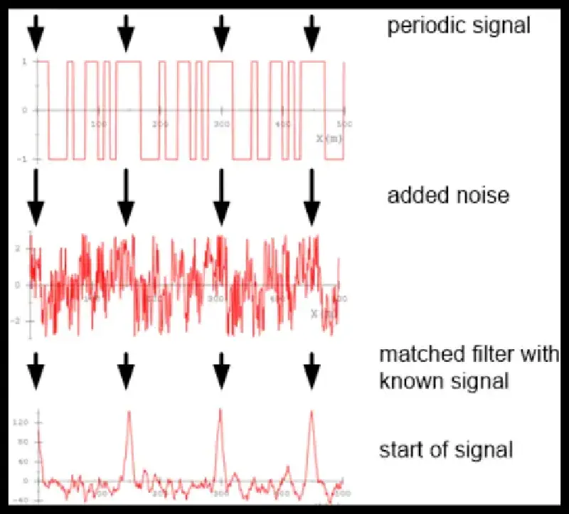
Here we handle the boundary with zeroes, but it can be done differently:

• for reflected, the leftmost $w_3$ would be $w_1 + w_3$ (along with the rightmost $w_1$)
• for periodic, the rightmost top cell would not be $0$ but $w_3$ instead (+ some others)

Here we’ve seen one of the major operations, convolution, the other being pooling:

• reduces the image resolution, done by merging several input pixels into one output pixel
• typically reduces $2 \times 2 \rightarrow 1$
• not sliding anymore, move by the window size instead (running window)
• usually either average pooling or max pooling

CNNs usually alternate between convolution, non-linear layers (ReLU), pooling, dropout layers, batch normalization layers and (towards the end of the network), fully-connected layers and softmax layers.

Receptive field of a neuron

• set of input pixels (from original image) that influence the value of a given neuron
• i.e. maximum size of detectable patterns
• RF of:
  • one convolutional layer is the size of the kernel
  • sequence of convolutional layers is additive (wrt. kernel radius)
  • pooling is multiplicative (wrt. pooling size)

Some history

• ImageNet (2008) ~14 mil. images, more than 1000 classes (224x224x3)
  • 1st public challenge (2010)
    • predict 5 guesses for the object class
    • correct if true label is within top 5 (“top-5 acc.”)
    • winner: non-linear SVM with hand-crafted features (28% top-5 error)
  • 2nd public challenge (2012)
    • winner: CNN AlexNet (15.3% top-5 error)
  • 3rd public challenge (2014)
    • winner: GoogLeNet – inception architecture (6.7% top-5 error)
    • runner-up: VGG – upscaling of LeNet (7.3% top-5 error)
      • clean and popular (compared to winner, which was quite hacky)
      • used as a comparison metric for things like Midjourney/DALL-E (FID score)
      • making VGG bigger did not work (vanishing gradient problem) – magnitude of gradient at the prompt decreases with the number of layers and the network doesn’t converge
  • 2015: Residual Network (ResNets)
    • instead of learning a function per layer, learn weights wrt. the input layer
    • also skip connections as identity mappings, preventing vanishing gradients
    • reaches superhuman performance (humans 4/5%, ResNet 3.6%)
    • for top-1, we they had 25% error (nowadays ~10%)
  • nowadays, use two tricks:
    • train on much larger datasets (up to 3B images)

Residual Networks (ResNet)

• base idea: use skip connections to avoid the vanishing grandient problem
• stages between pooling layers (image resolution unchanged within the stage)
• block – sequence of layers + one skip connection (bridges the block):
  • batch normalization: adjust mean and variance of pre-activations
    • bad when pre-activations have an arbitrary mean and variance (data should be within the intersting region of the activation function)
    • ($\mu, \sigma$) calculated for each batch
• layers – do the actual work

Training

• rule of thumb: more data is better (nowadays $3 \times 10^9$ images)

Data augmentation

• apply transformations to the data that keeps the classification unchanged
• artificially increases the dataset
• popular augmentations:
  • geometric distortions:
    • mirroring, 90deg rotations
    • shearing % small angle rotations
    • crop regions & resize to original size
  • image quality distortions:
    • add noise – Gaussian / salt & pepper (random 0/1 pixels)
    • mash out regions (set to gray)
  • color distortions:
    • transform to gray
    • transform color space (eg. LAB)
  • other distortions:
    • edge detection (human should still recognize it)
• hyperparameters:
  • amount of distortion
  • number of simultaneous distortions ($\ge 2$ works good)

Self-supervised training

• use augmentation to avoid manual labelling
• strategy (1): use augmentation that can be labeled automatically
  • rotate by $\alpha \implies$ predict $\alpha$
  • to solve this, network learns features that are useful for other tasks – cut out the angle detection and use the reset of the network for feature detection
• strategy (2): contrastive learning
  • present augmented pairs; if it originated from the same image, features should be similar, else they should be different (ie. ignore data augmentations)
  • SIMCLR network – famous for doing this
• strategy (3): semi-supervised learning
  • subset of the training set is labeled and rest is unlabeled
  • student-teacher approach:
    • train the teacher from the labeled and then use the teacher to label the unlabeled (preferably soft labels since it can make mistakes and might not be sure)
    • train the student with the original and the pseudolabels
    • experimentally, often the student is better / has a smaller network

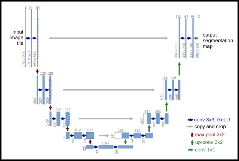
U-Net

• tasks in image analysis:
  1. classification (what we were talking about), 1 label per image
  2. instance classification & segmentation, 1 label + bounding box per instance
  3. semantic segmentation, 1 label per pixel (one-hot vector per pixel)
     • less difficult than (2), since objects can be occluded by others
• U-Net solves (3)
• has the name because it looks like the letter U
• idea: coarsening to detect the semantics + refinement for pixel-precision

• variation: nnU-Net (2021)
  • designed here in Heidelberg!
  • previously, people designed new net for every task
  • observation: have rules to design the network given the task (nn = no new)
  • won about 30 medical benchmark competitions
• U-net is a specific example of an auto-encoder:
  • takes in a $D$-dimensional data
  • then uses an encoder to convert to $C$-dimensional codes
  • lastly uses a decoder to convert back to the ~original data
  • since $D \gg C$, this is lossy, but works really well
  • we want to minimize $(X - \mathrm{D}(\mathrm{E}(X)))^2$

Regression

• features $X$, response $Y$ real-valued scalar (or vector)
  • compared to classification where $Y$ is discrete
• predict $Y$ deterministically ($Y = f_{\theta}(x)$) or stochastically ($y \sim p_\theta (Y \mid X)$)
• functional representation lemma (aka “reparametrization trick” / “noise outsourcing”)
  • every conditional probability $p(Y \mid X)$ can be expressed by a deterministic function & independent noise: $$y \sim p(Y \mid X = x) \equiv y = f_\theta(x, \varepsilon)$$ with $\varepsilon$ drawn from a distribution (usually Gaussian) independent from $X$; eg. $$y \sim \mathcal N(Y, \mu(x), \Sigma(x)) \equiv y = \mu(x) + \Sigma(x)^{1/2} \cdot \varepsilon \qquad \varepsilon \sim N(0, \mathbf{I})$$
  • much more convenient since the distribution is fixed (not dependent on $X$)

Linear regression

• easy case, just like linear regression
• assume that data is generated by some true (but unknown) generative process
  • in this case linear model with additive Gaussian noise, for simplicity assume $y \in \mathbb{R}$ $$Y_i = X_i \beta^* + b^* + \varepsilon_i \qquad \varepsilon_i \sim \mathcal N(0, \sigma^2)$$ (i.e. variance is fixed but unknown)
• given $\mathrm{TS} = \left\{(X_i Y_i)\right\}_{i = 1}^N$, find $\hat \beta \approx \beta^*$ and $\hat b = b^*$
• important: assume that only $Y$ is noisy, not $X$ (other variant also exists)

• derive loss by maximum likelyhood principle and i.i.d. assumption: $$\begin{aligned} \hat\beta, \hat b = \argmin_{\beta, b} p(\mathrm{TS}) &= \argmax_{\beta, b} \prod_{i = 1}^{N} p(Y_i \mid X_i) \\ &= \argmin_{\beta, b} \sum_{i = 1}^{N} -\log p(Y_i \mid X_i) \\ &= \argmin_{\beta, b} \sum_{i = 1}^{N} -\log N(Y_i \mid X_i \beta + b = \mu(x), \sigma^2) \\ &= \argmin_{\beta, b} \sum_{i = 1}^{N} -\log \frac{1}{\sqrt{2 \pi \sigma^2}} \exp\left(-\frac{1}{2} \frac{(Y_i - X_i \beta - b)^2}{\sigma^2}\right) \\ &= \argmin_{\beta, b} \sum_{i = 1}^{N} \left[\cancel{\log \sqrt{2 \pi \sigma^2}} + \cancel{\frac{1}{2}} \frac{\left(Y_i - X_i \beta - b\right)^2}{\cancel{\sigma^2}}\right] \\ &= \boxed{\argmin_{\beta, b} \sum_{i = 1}^{N} \left(Y_i - X_i \beta - b\right)^2} \\ \end{aligned}$$

• squared loss $\implies$ ordinary least squares (OLS) regression
• can be solved analytically: $$\frac{\partial \mathcal{loss}}{\partial b} = \sum_{i = 1}^{N} -2 \left(Y_i - X_i \beta - b\right) \overset{!}{=} 0\\ \Downarrow \\[0.5em] b = \underbrace{\frac{1}{N} \sum_{i = 1}^{N} Y_i}_{\bar Y} - \underbrace{\left(\frac{1}{N} \sum_{i = 1}^{N} X_i\right)}_{\bar X}\beta$$

Written another way, we get $$\bar y = \bar X \beta + \hat b$$ meaning that the regression always goes through the center of mass of TS, which allows us to first center the data ($X - \bar X, Y - \bar Y$), making the center of mass the origin and getting rid of $\hat b$ (same as classification).

$$\frac{\partial \mathcal{loss}}{\partial \beta} = \sum_{i = 1}^{N} -2 (Y_i - X_i \beta) X_i^T \overset{!}{=} 0 \\ \Downarrow \\[0.5em] \boxed{\beta = \frac{\sum_{i = 1}^{N} Y_i X_i^T}{\sum_{i = 1}^{N} X_i X_i^T}}$$

Now we want to generalize to feature vectors – $X_i \in \mathbb{R}^{1 \times D}$ (row vector) $\implies$ rewrite the objective in matrix form (still assume centered data):

$$\hat \beta = \argmin_\beta \sum_{i = 1}^{N} (Y_i - X_i \beta)^2 = \argmin_\beta (Y - X \beta)^T (Y - X\beta)$$ where $Y \in \mathbb{R}^{N \times 1}, X \in \mathbb{R}^{N \times D}$, so we get $$\frac{\partial \mathcal{loss}}{\partial \beta} = 2 (Y - X \beta) X^T \\ \Downarrow \\[0.5em] \boxed{(X^T X) \hat \beta = X^T Y}$$

which are called the normal equations of the OLS problem, since $\beta$ is the normal of the regression plane and we can solve it as $$\boxed{\hat \beta = \underbrace{(X^T X)^{-1} X^T}_{\text{pseudoinverse}\ X^+} Y}$$

Pseudoinverse is a generalization of the inverse for rectangular matrices:

• not a great way to calculate this – expensive and also $X^T X$ might be too degenerate
  • if at least one feature (column of $X$) can be expressed as a linear combination of other features, it will be entirely degenerate and OLS will have no solution
• contition number $\kappa(X) = ||X|| \cdot ||X^+||$ measures this:
  • if $\kappa(x) = 1 \implies X$ is nice (almost orthogonal features)
  • if $\kappa(x) \gg 1 \implies X$ has almost redundant features, $\hat \beta$ becomes inaccurate
  • if $\kappa(x) = \infty \implies X$ has redundant features, $\hat \beta$ doesn’t exist
    • infinity arrises from the norm of $X^+$ (division by $0$)

We can instead solve OLS by SVD:

• every matrix $X$ can be decomposed into $X = U \Lambda V^T$ for
  • $V \in \mathbb{R}^{D \times D}$ orthonormal matrix
  • $\Lambda \in \mathbb{R}^{D \times D}$ diagonal matrix
  • $U \in \mathbb{R}^{N \times D}$ quasi-orthonormal matrix
• using this we get $$\boxed{\beta = (V \Lambda^{-1} U^T) Y}$$
  • if $k$ features are redundant, $k$ eigenvalues are $0$
  • when we’re doing $\Lambda^{-1}$, this explores, set $\Lambda' = \frac{1}{0} \mapsto 0$
  • this gives us the minimum norm solution of the degenrate OLS problem
• condition number for SVD is $\kappa(X) = \frac{\max \lambda}{\min \lambda}$
• advantage: numerically very stable, even when $X$ is almost degenerate
• disadvantage: very complicated algorithm (500 LOC of Fortran); nowadays this is ok

Third solution: QR decomposition

• much easier than SVD, reasonably robust for bad data
• uses a different decomposition $X = Q \cdot R$ for
  • $Q \in \mathbb{R}^{N \times D}$ orthonormal
  • $R \in \mathbb{R}^{D \times D}$ upper triangular
• using this, we get $$\boxed{\hat \beta R^{-1} Q^T Y} \quad \text{or alternatively} \quad \boxed{R \hat\beta = Q^T Y}$$ which can be solved by a simple algorithm – $R$ is upper triangular so we can use substitution from the last row of $R \hat\beta$ upward

What do we do if $N$ and $D$ are very big?

• in theory, we’re screwed (SVD complexity $\mathcal{O}(N \times D^2)$)
• in practice, big $X$ matrices usually have special structure which we can exploit
  • $X$ sparse – alg. only deals with the non-zero elements
  • $X$ is a convolution – even more strict
• we don’t access $X$ directly, but via subroutines
  • vector-matrix product $b^T X \implies \mathtt{vector\_times\_X}(b)$
  • matrix-vector product $Xa \implies \mathtt{X\_times\_vector}(a)$
  • all the tricks to exploit the special strucure of $X$ hidden here:

LSQR

1. trick: only use the subroutines to exploit the structure
2. trick: rearrange the computation such that only 2 rows or columns of the result matrices are needed simultaneously (in memory)

• LSQR decomposition is $X = U \cdot B \cdot V^T$ where
  • $U \in \mathbb{R}^{N \times D}$ is orthonormal
  • $B \in \mathbb{R}^{D \times D}$ is upper bi-diagonal
    • diagonal + one more diagonal above are non-zero, the rest is zero
  • $V \in \mathbb{R}^{D \times D}$ is orthonormal
• implemented as scipy.sparse.linalg.lsqr in Python (or new and improved lsmr)
  • arguments are sparse matrices

The lecture here has an interlude into computer tomography, which can be solved using least-squares. Most of it is explained in homework 4 so I’m not going to repeat it here.

Least Squares v2.0

What do we do when noise variance is not constant?

• i.e. we change the generative model into $$Y_i = X_i \beta^* \underbrace{(+ b)}_{\text{0}} + \varepsilon_i \qquad \varepsilon_i \sim N(0, \sigma_i^2)$$
• data still independent but no longer identically distributed
• we use $\theta$ since we want to learn both $\beta$ and $\sigma$

$$\begin{aligned} \theta = \argmax_\theta p(\mathrm{TS}) &= \argmax_\theta \prod_{i = 1}^{N} p_i(Y_i \mid X_i) \\ &= \argmin_\theta \sum_{i = 1}^{N} - \log p_i(Y_i \mid X_i) \\ &= \argmin_\theta \sum_{i = 1}^{N} - \log N(Y_i - X_i \beta \mid 0, \sigma_i^2) \\ &= \argmin_\theta \sum_{i = 1}^{N} \left[-\log \frac{1}{\sqrt{2 \pi \sigma_i^2}} + \frac{\left(Y_i - X_i \beta\right)^2}{2 \sigma_i^2} \right] \\ &= \boxed{\argmin_\theta \sum_{i = 1}^{N} \left[\cancel{\frac{1}{2}}\log \sigma_i^2 - \cancel{\frac{1}{2}} \frac{\left(Y_i - X_i \beta\right)^2}{\sigma_i^2} \right]} \end{aligned}$$

Here we distinguish multiple cases:

1. OLS (all $\sigma$s are the same) – we can simplify further and get stuff from lectures above
2. weighted LS ($\sigma_i$ are known) – then $$\argmin_\beta \sum_{i = 1}^{N} \frac{(Y_i - X_i \beta)^2}{\sigma_i^2}$$
   • the $\sigma$s act as weights for the residuals
   • we can rewrite in matrix notation ($\sigma$s as a diagonal) and get $$\hat \beta = \argmin_\beta (Y - X \beta)^T \Sigma^{-1} (Y - X \beta)$$
   • this can be solved by setting the derivative to zero and we get a weighted pseudo-inverse $$\boxed{\hat \beta = \left(X^T \Sigma^{-1} X\right)^{-1} X^T \Sigma^{-1} Y}$$
3. iteratively reweighed LS ($\sigma_i$ are not constant and unknown) – learn the $\sigma$s jointly with $\beta$)
   • $\sigma_i$ is unsupervised, $\beta$ is supervised – gives rise to interesting algorithms
   • the problem can be formulated as $$\argmin_\theta \sum_{i = 1}^{N} \left[\log \sigma_i^2 - \frac{\left(Y_i - X_i \beta\right)^2}{\sigma_i^2} \right]$$ usually called David-Sebastian score or hetero-scedastic loss
   • if $(Y_i - X_i \beta)^2$ is big $\implies$ increase $\sigma_i$ to make the loss smaller, but we pay the penalty of $\log \sigma_i^2$ for big $\sigma$s (optimal solution selects $\sigma_i^2$ for the best trade-off)

Alternating optimization

• we want to solve IRLS by alternating learning $\beta$ and $\sigma$
• two groups of parameters $\theta = \left[\theta_1, \theta_2\right]$ (here $\theta_1 = \beta, \theta_2 = \left\{\sigma_i^2\right\}_{i = 1}^N$)
• main idea: optimize $\theta_1$ while keeping $\theta_2$ fixed (and vice versa)

1. define initial guess for $\theta_2^{(0)}$
2. for $t = 1, \ldots, T$ (or until convergence)
   • optimize $\theta_1^{(t)}$, keeping $\theta_2^{(t - 1)}$ fixed
   • optimize $\theta_2^{(t)}$, keeping $\theta_1^{(t)}$ fixed

• benefit: individual optimization problems are much easier (can have an analytic solution)
• drawback: usually doesn’t converge to the global optimum

To solve IRLS using this method, we do the following

1. define initial guess as $\tau_i = 1$ ($\tau_i = \sigma_i^2$
2. for $t = 1, \ldots, T$ (or until convergence)
   • obtain $\beta^{(t)}$ via weighted least squares (since $\sigma$s are known and fixed)
   • since $\beta$ is fixed, we get $$\left\{\tau_i^{(t)}\right\} = \argmin_{\left\{\tau_i\right\}} \sum_{i = 1}^{N} \frac{Y_i - X_i \beta^{(t)}}{\tau_i} + \log \tau_i$$ which we can solve by setting the derivative to $0$ and obtain $$\boxed{\tau_i^{(t)} = (Y_i - X_i \beta^{(t)})^2}$$ i.e. standard derivations are equal to the magnitude of the error

How many iterations are required?

• in theory (with infinite accuracy) two iterations are sufficient
• in practice few iterations are sufficient (kinda cool, no?)

Regularized regression

• even if we don’t have a unique solution, we can select the “best” one
• we already saw penalties $||\beta^2||$ in SVM and $\log \sigma_i^2$ in IRLS
• we need regularization in two cases
  1. more features than observations ($D > N$)
  2. condition of matrix $X$ is bad ($\kappa(X) \gg 1$)o
     • features are almost redundant, $\hat \beta$ tends to overfit
     • assume feature $j$ and $j'$ are identical in TS ($X_j = X_{j'}$)
     • if $\hat \beta$ is a solution, so it $\hat \beta'$ with $\hat \beta_j' = \hat \beta_j' + \gamma$ and $\hat \beta_j' = \hat \beta_j' - \gamma$
     • this also works for very large $\gamma$, which is a problem since the features might be different in test instances (i.e. overfitting)
     • in practice, usually more features and only near cancelation

Ridge regression

Uses a standard regularization idea to penalize $\beta_j$ with large magnitude (or squared magnitude):

$$\hat \beta = \argmin_\beta (Y - X\beta)^T (Y - X\beta) \quad s.t. \quad ||\beta^2|| \le t$$

• if constraint doesn’t activate after we solve, we’re chilling
• otherwise add the constraint as a Lagrange multiplier (same as SVM)

$$\hat \beta_{RR} = \argmin_\beta (Y - X\beta)^T (Y - X\beta) + \tau ||\beta^2||$$

Setting the derivative to zero, we obtain the regularized pseudo-inverse $$\hat \beta_{RR} = (X^T X + \tau \mathbb{I})^{-1} X^T Y$$

• data should ideally be standardized (zero mean, unit variance) so we shrink $\tau$ equally

Alternative solution via augmented feature matrix – reduces to OLS by modifying $X$ and $Y$ to be $$\tilde X = \begin{pmatrix} & X & \\ & & \\ \sqrt{\tau} & & \\ & \ddots & \\ & & \sqrt{\tau} \\ \end{pmatrix} \qquad \tilde Y = \begin{pmatrix} Y \\ 0 \\ \vdots \\ 0 \end{pmatrix}$$

• by expanding OLS, we can see this is equivalent to original loss

Another alternative solution is via SVD.

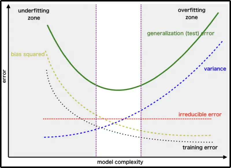
Bias-variance trade-off

When using regularization, we’d like to know two things:

1. what’s the price that we pay for regularization?
2. how to choose $\tau$ to minimize disadvantages

Both solved via bias-variance trade-off: we have $M$ teams working on the same problem, each with their own $\mathrm{TS}$:

• how much will the results differ between teams?
• what happens when $M \rightarrow \infty$?

Definitions:

• $\beta^*$: weights of the true generative process $Y^* = X \beta^* + \varepsilon$
• $\hat \beta_m$: results of team $m$
• $\mathbb{E}_m [\hat \beta_m] \approx \frac{1}{M} \sum_{m = 1}^{M} \hat \beta_m$: average result of all teams
• $\mathrm{Cov(\hat \beta_m}) = \mathbb{E}_m \left[\left(\hat \beta_m - \mathbb{E}[\hat \beta_m]\right)\left(\hat \beta_m - \mathbb{E}[\hat \beta_m]\right)^T\right]$:
• $\mathrm{bias} = \beta^* - \mathbb{E}_m [\hat \beta_m]$: systematic error after combining team results

Now we’ll measure the quality of outcomes by $$\begin{aligned} \mathrm{MSE} &= \mathbb{E}_m \left[\left(\hat \beta_m - \beta^*\right)^2\right] \\ &= \mathbb{E}_m \left[\left(\hat \beta_m - \mathbb{E}[\hat \beta_m] + \mathbb{E}[\hat \beta_m] + \beta^*\right)^2\right] \\ &= \underbrace{\mathbb{E}_m \left[\left(\hat \beta_m - \mathbb{E}_m (\hat \beta_m)\right)^2\right]}_{\text{covariance}} + \underbrace{\mathbb{E}_m \left[\left(\beta^* - \mathbb{E}_m [\hat\beta_m]\right)^2\right]}_{\text{bias}^2} \\ \end{aligned}$$

Useful, because we can see that $\tau$ (regularization) has opposite effects on bias and variance – “bias-variance trade-off”

• $\tau = 0 \ldots$ high variance (teams disagree) but zero bias
• $\tau = \infty \ldots$ all teams same solution, but it’s $0$
• $\tau > 0 \ldots$ agreement between teams increases but so does bias (trade-off)

• best trade-off: all error sources have roughly same magnitude
  • check via cross-validation (or validation set)
• bad: only address a single error source (diminishing returns)

Other regularization terms

• Ridge regression: regularization term $$||\beta||_2 = \sum_{i = 1}^{D} \beta_j^2 \le t$$
• Feature selection: $$||\beta||_0 = \sum_{i = 1}^{D} \mathbb{1}[\beta_j \neq 0] \le t$$
  • count how many features are active
  • advantage: reduce the number of measurements
  • disadvantage: finding the optimal feature set is NP-hard (but in practice a simple greedy algorithm like OMP is often good enough)
• LASSO regression: $$||\beta||_1 = \sum_{i = 1}^{D} |\beta_j| \le t$$
  • stands for Last Absolute Shrinkage Selection Operator
  • also performs feature selection when $t$ is small enough
  • advantage:
    • still a convex optimization problem $\implies$ unique solution
    • solution often sparse (many $\beta_j = 0$) $\implies$ feature selection
  • disadvantage:
    • bias (bias-variance trade-off)
    • active set may not be as sparse as in $L_0$ optimization
  • many algorithms (in the field of linear optimization)
    • gradient descent
    • LARS (Least Angle RegreSsion) algorithm – almost the same as OMP, but at the beginning of each iteration, checks if the matrix is redundant (and removes weakest factors until it isn’t); doesn’t happen too often though

Orthogonal Matching Pursuit (OMP)

• approximately (local optimum) solves feature selection, i.e. $$\hat \beta = \argmin_\beta \sum_{i = 1}^{N} (Y_i^* - X_i \beta)^2 \quad \text{s.t.} ||\beta_0|| \le t$$

1. initialization: set of active features$A^{(0)} = \emptyset$
2. for $\tau = 1, \ldots, t$ (max. number of features)
   • compute residual of current guess $R = Y^* - X \beta^{(\tau - 1)}$
   • find best inactive feature $j^{(\tau)} = \argmax_{j \not\in A^{(\tau - 1)}} |X_j^T R|$
     • if the direction of the new feature is similar to the residual, it improves the solution by a lot
     • if it’s orthogonal then it can’t do much
   • add new feature to active set $A^{(\tau)} = A^{(\tau - 1)} \cup \left\{j^{(\tau)}\right\}$
   • compute new guess by solving OLS only with active features

Non-linear regression

• keep squared loss $\implies \hat \theta = \argmin_\theta \sum_{i = 1}^{N } \left(Y_i^* - f_\theta (X_i)^2\right)$
  • $f_\theta(X) = X \beta \implies$ linear regression
  • $f_\theta(X)$ neural network with parameters $\theta$
• true generative process $Y_i^* = f_{\theta^*} (X_i) + \varepsilon_i \quad \varepsilon_i ~ N(0, \sigma^2)$

Two general approaches:

1. transform features such that we can run linear regression (and use OLS)
   • hand-crafted
   • learned (first layer of a NN learns the parameters) - same as classification, except
     • squared loss (instead of cross-entropy)
     • last layers is linear (no activation)
2. design algorithms to solve non-linear least squares
   • if $\dim(\theta)$ is not very high ($\mathcal{O}(100)$), use Levenberg-Markquart
   • regression trees and forests / Gaussian processes
     • good results if $\mathrm{TS}$ is small (so NN cannot be trained)

I missed a few lectures here, the notes of the next chapter are taken from the recording of the last year’s “Fundamentals of Machine Learning class”.

Decision trees / forests

• idea: approximate a function using piecewise constant function
• in theory, we can get an arbitrarily good approximation

How to choose bins?

• classical: grid (great for $D = 1, 2$, rather expensive for $D \ge 3$)
• better: define bins adaptively (bin size based on the number of datapoints)
  1. method: $k$-means (defines bins by nearest-neighbour computation)
  2. method: recursive subdivision (what we’ll be doing)

For regression/classification, we can build a tree on top of it by doing the following:

Algorithm (generic tree building):

1. create the root note with all data
   • also put all of the data on the stack
2. while the stack is not empty:
   • take the top node
   • check if the termination criterion is reached
     • create a leaf node which stores the desired prediction
   • otherwise
     • find the best possible split and create 2 children
     • put the data in the respective child
     • put the children on the stack

For specific problems:

• termination criteria
  • generic:
    • stop at a defined depth (hyperparameter)
    • stop at a defined number of instances in a node (hyperparameter)
  • application-specific:
    • classification: all instances in the node have the same label (then we don’t improve by splitting further) – we say they are pure
• split criteria:
  • axis-aligned, then decide left/right child by a 1-D threshold
  • oblique splits (compute a new feature as a linear combination): sometimes more accurate but also more expensive
  • we usually restrict possible thresholds to the midpoint between neighbouring instances – then for $N_m$ instances and $D$ features we have $N_m \cdot D$ splits
    • exhaustive search to find the best one (given a score function) or
    • restrict the search to a random subset of features (eg. $\sqrt{D}$)

For classification trees:

• the prediction is the majority class in the leaf node
• the split criterion prefers splits that separate classes well… given a node $m$:
  • C4.5 algorithm: measure the entropy by iterating over all classes: $$H_m = -\sum_{k = 1}^{C} \hat p_{m, k} \log \hat p_{m, k} \qquad \hat p_{m, k} = \frac{N_{m, k}}{N}$$
  • CART algorithm: uses Gini impurity: $$G_m = 1 - \sum_{k = 1}^{C} \hat p_{m, k}^2$$
  • in either case, the loss of a given split is $N_l H_l + N_r H_r$ (or $G$ if we use CART)

For classification trees:

• the prediction is the average value
• the split criterion minimizes the squared loss… given a node $m$:
  • the average is $\hat y_m = \frac{1}{N_m} \sum_{i \in m} y_i$ so we get $\mathcal{loss} = \sum_{i \in m} (y_i - \hat y_{m})^2$
  • the loss of a given split is the sum of the squared losses

Since trees tend to overfit, we can train several trees (i.e. forests). They have to be different for which there are a few tricks:

• in each node, consider a different random subset of features (we’re doing this)
• train each tree on a different random subset of the training set: bootstrapping:
  • create a new $\mathrm{TS}'$ by uniform sampling with replacement ($\mathrm{TS}'$ is initially empty, then add $N$ random instances)