slama.dev

Mining Massive Datasets

notes · 8. 2. 2023 · [edit]

• Lecture overview
• Programming and Frameworks
  • PySpark
    • RDDs [cheatsheet]
    • DataFrames [cheatsheet]
    • ML with Spark
    • Spark Streaming
• Recommender Systems
  • Collaborative filtering (CF)
    • User-user CF
    • Item-item CF
    • Pros/Cons
  • Content-based recommendations
    • Pros/Cons
  • Latent factor models
• Link Analysis
  • Flow formulation
  • Matrix formulation
  • Practical computation
  • Topic-Specific PageRank
  • TrustRank
• Locality Sensitive Hashing
  • Preface
  • Shingling
  • Min-hashing
  • Locality-Sensitive Hashing
• Association Rule Discovery
  • A-Priori Algorithm
  • PCY Algorithm
• Online Advertising
• Mining Data Streams
  • Stream Filtering
    • First-cut solution
    • Bloom filter
  • Stream Sampling
    • Fixed portion
    • Fixed size (Reservoir Sampling)
  • Stream Counting
    • Flajolet-Martin
    • AMS Algorithm

Preface

This website contains my lecture notes from a lecture by Artur Andrzejak from the academic year 2022/2023 (University of Heidelberg). If you find something incorrect/unclear, or would like to contribute, feel free to submit a pull request (or let me know via email).

Note that the notes only cover the topics required for the exam, which are only a portion of the contents of the lecture.

Lecture overview

1. Spark architecture and RRDs [slides]
2. Spark Dataframes + Pipelines [slides]
3. Recommender Systems 1 [slides]
4. Recommender Systems 2 [slides]
5. Page Rank 1 [slides]
6. Page Rank 2 [slides]
7. Locality Sensitive Hashing 1 [slides]
8. Locality Sensitive Hashing 2 [slides]
9. Frequent itemsets + A-Priori algorithm [slides]
10. PCY extensions [slides]
11. Online bipartite matching + BALANCE [slides]
12. Mining data streams 1 [slides]
13. Mining data streams 2 [slides]

Programming and Frameworks

PySpark

RDDs [cheatsheet]

Main data structure are RDDs (resilient distributed datasets):

• collection of records spread across a cluster
• can be text line, string, key-value pair, etc.

Two operation types:

• transformations: lazy operations to build RDDs from other RDDs
• actions: return a result or write it to storage

DataFrames [cheatsheet]

PySpark’s other main data structure are DataFrames:

• table of data with rows and (named) columns
• has a set schema (definition of column names and types)
• lives in partitions (collections of rows on one physical machine)

ML with Spark

• mainly lives in MLlib, which consists of
  • pyspark.ml (high-level API) and
  • pyspark.mllib (low-level API)
• is based on pipelines, which set up everything, including
  • data cleaning
  • feature extraction
  • model training, validation, testing
  • they use DataFrames

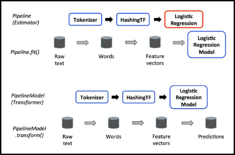
Definition (Transformer): an algorithm which transforms one DataFrame into another

• uses a transform() method to activate (i.e. transform the DataFrame)

Definition (Estimator): an algorithm which can be fit on a DataFrame to produce a Transformer

• abstracts the concept of a learning algorithm
• contains a fit() function, which when call produces a Transformer

Definition (Pipeline): an object which contains multiple Transformers and Estimators

• a complete untrained pipeline is an Estimator
• after calling fit(), all estimators become transformers!

Spark Streaming

General idea is to:

• split the stream into batches of $X$ seconds,
• perform RDD operations and lastly
• return the results of the RDD operations in batches

DStream (discretized stream) – container for a stream, implemented as a sequence of RDDs

# an example that returns the word counts in a stream

# 2 threads - source feed + processing
sc = SparkContext("local[2]", "NetworkWordCount")

# batch interval = 1s
ssc = StreamingContext(sc, 1)

# DStream will be connected here
lines = ssc.socketTextStream("localhost", 9999)

# lines is an RDD (kinda) and we can behave as such
words = lines.flatMap(lambda line: line.split(" "))
pairs = words.map(lambda word: (word, 1))
wordCounts = words.reduceByKey(lambda x, y: x + y)

wordCounts.pprint()

# start the task and wait for termination
ssc.start()
ssc.awaitTermination()

Recommender Systems

Problem: set of customers $X$, set of items $I$, utility function (set of ratings) $u: X \times I \mapsto R$

• $R$ usually $\in [0, 1]$
• can be stored in a utility matrix:

Note: for some reason, this matrix is $I \times X$ while all other notation is $X \times I$ (like $r_{xi}$, for example). It’s confusing, I’m not sure why we’ve defined it this way.

Goal: extrapolate unknown ratings from the known ones.

Collaborative filtering (CF)

Idea: take known ratings of other similar items/users.

User-user CF

• find set $N$ of other users whose ratings are similar to user $x$’s ratings
• estimate $x$’s ratings based on ratings of users from $N$

Algorithm:

1. let $r_x$ be vector of user $x$’s ratings and $N$ the set of neighbors of $x$
2. predicted rating of user $x$ for item $i$ is $$\underbrace{r_{xi} = \frac{1}{|N|} \sum_{y \in N} r_{yi}}_{\text{naive version (just average)}} \qquad \underbrace{r_{xi} = \mathrm{avg}(r_x) + \frac{\sum_{y \in N} \mathrm{sim}(x, y) \cdot (r_{yi} - \mathrm{avg}(r_y))}{ \sum_{y \in N} \mathrm{sim}(x, y)}}_{\text{improved, takes similarity of users into account, along with their bias}}$$

To calculate similarity, we can use a few things:

• Cosine similarity measure (angle between vectors) $$\mathrm{sim}(x, y) = \mathrm{cos}(r_x, r_y) = \frac{r_x \cdot r_y}{ ||r_x|| \cdot ||r_y||}$$
  • where $||x|| = \sqrt{\sum_{i = 0}^n x_i^2}$
  • problem 1: missing ratings become low ratings
  • problem 2: doesn’t account for bias (some users rate higher on average)
• Pearson similarity measure (angle between normalized + offset vectors without zero entries) $$\mathrm{sim}(x, y) = \frac{\sum_{s \in S_{xy}} (r_{xs} - \mathrm{avg}(r_x)) (r_{ys} - \mathrm{avg}(r_y))}{\sqrt{\sum_{s \in S_{xy}} \left(r_{xs} - \mathrm{avg}(r_x)\right)^2} \sqrt{\sum_{s \in S_{xy}} \left(r_{ys} - \mathrm{avg}(r_y)\right)^2}}$$
  • where $S_{xy}$ are the indexes that are non-zero for both $x$ and $y$
  • problem 1 fixed by only taking items rated by both users
  • problem 2 fixed by offsetting by average

This way of writing Pearson is hiding what’s really going on, so here is a nicer way: let $s_x$ and $s_y$ be formed from vectors $r_x, r_y$ by removing the indexes where either one is zero. Then the Pearson similarity measure can be calculated like such: $$\mathrm{sim}(r_x, r_y) = \cos(s_x - \mathrm{avg}(r_x), s_y - \mathrm{avg}(r_y))$$

To calculate neighbourhood, we can do a few things:

• set a threshold for similarity and only take those above
• take the top $k$ similar users, whatever their similarities are

Item-item CF

Analogous to User-user: for rating item $i$, we’re find items rated by user $x$ that are similar (as in rated similarly by other users). To do this, we can again use $\mathrm{sim}$, obtaining $$r_{xi} = \frac{\sum_{j \in N} \mathrm{sim}(i, j) \cdot r_{xj}}{\sum_{j \in N} \mathrm{sim}(i, j)}$$

The improved version has a slightly different baseline to User-User, namely $$r_{xi} = b_{xi} + \frac{\sum_{j \in N} \mathrm{sim}(i, j) \cdot (r_{xj} - b_{xj})}{\sum_{j \in N} \mathrm{sim}(i, j)}$$ where $b_{xi} =$ mean item rating $+$ rating deviation of user $x$ $+$ rating deviation of item $i$.

Pros/Cons

• [+] Works for any kind of item (no feature extraction)
• [-] Cold start (needs user data)
• [-] Sparsity (user/rating matrix is sparse)
• [-] First rater (can’t recommend an item that hasn’t been rated)
• [-] Popularity bias (tends to recommend popular items)

Content-based recommendations

Main idea: create item profiles for each item, which is a vector $v$ of features:

• author, title, actor, director, important words
• can be usually encoded as a binary vector with values getting fixed positions in the vector
  • can also be mixed (binary encoding + floats where appropriate) $$i_1 = ( \underbrace{1, 0, 0, 1, 0}_{\text{set of actors}}, \ldots, \underbrace{0, 0, 1, 1, 0}_{\text{set of directors}}, \ldots, \underbrace{3.2, 2.9, 2.7, 1.3, 5.0}_{\text{ratings from movie databases}}, \ldots)$$

For creating user profiles, we can do a weighted average (by rating) of their item profiles: $$x = \left(r_1 i_1 + r_2 i_2 + \ldots + r_n i_n\right) / n$$

For matching User and Item (i.e. determining rating), we can again use cosine similarity between the user profile and the item.

Pros/Cons

• [+] No need for user data (no cold start or sparsity)
• [+] Can recommend new + unpopular items
• [+] Able to provide explanations (why was that recommended?)
• [-] Finding good features is hard
• [-] Recommendations for new users
• [-] Overspecialization – unable to exploit quality judgement from other users

Latent factor models

Merges Content-Based Recommenders (rating is a product of vectors) and Collaborative filtering (weighted sum of other ratings from the utility matrix) – use user data to create the item profiles! We’ll do this by factorizing the matrix into user matrix $P$ and item matrix $Q$ such that we minimize SSE $$\min_{P, Q} \sum_{\left(i, x\right) \in R} (r_{xi} - q_{i} \cdot p_x)^2$$

What we want to do is split the data into a training set, which we use to create the matrices, and the testing set, on which the matrices need to perform well. To do this well, we’ll use regularization, which controls for when the data is rich and when it’s scarce (lots of zeroes in $p_x$s and $q_i$s): $$\min_{P, Q} \underbrace{\sum_{\left(x, i\right) \in R} \left(r_{xi} - q_i p_x\right)^2}_{\text{error}} + \underbrace{\lambda_1 \sum_{x} ||p_x||^2 + \lambda_2 \sum_{i} ||q_i||^2}_{\text{„length“ (approx. num. of non-zeros in p, q)}}$$ for $\lambda_1, \lambda_2$ user-set regularization parameters.

Link Analysis

Flow formulation

Problem: we have pages as a directed graph. We want to determine the importance of pages based on how many links lead to it. I.e. if page $j$ of importance $r_j$ has $n$ outgoing links, each link gets importance $r_j / n$. Formally: $$r_j = \sum_{i \rightarrow j} \frac{r_i}{ d^{\mathrm{out}}_i}$$

Can be expressed as a system of linear equations to be solved (Gaussian elimination).

Matrix formulation

Can also be formulated as an adjacency matrix $M$, $$M_{ji} = \begin{cases} \frac{1}{d^{\mathrm{out}}_i} & \text{edge}\ i \rightarrow j \\ 0 & \text{otherwise} \end{cases}$$ then we can define the flow equation as $$Mr = r$$ meaning that we’re looking for the eigenvector of the matrix. Since the matrix is stochastic (columns sum to 1), its first eigenvector has eigenvalue 1 and we can find it using power iteration (see the PageRank formulation below).

This, however, has two problems:

• dead ends (when a page has no out-links); makes the matrix non-stochastic!
• spider traps (when there is no way to get out of a part of the graph)

Both are solved using teleports – during each visit, we have a probability of $1 - \beta$ to jump to a random page ($\beta$ usually $0.8$). In a dead-end, we teleport with probability $1$.

Using this, we get the Google PageRank equation: $$\underbrace{r_j = \sum_{i \rightarrow j} \beta \frac{r_i}{d^{\mathrm{out}}_i} + (1 - \beta) \frac{1}{N}}_{\text{PageRank equation}} \qquad \underbrace{A = \beta M + (1 - \beta) \left[\frac{1}{N}\right]_{N \times N} \quad Ar = r}_{\text{Google Matrix A}}$$

Practical computation

To reduce the matrix operations, we can rearrange the matrix equation and get $$r =\beta M \cdot r + \left[\frac{1 - \beta}{N}\right]_N$$

Algorithm (PageRank):

• set $r^{\mathrm{old}}_j = \frac{1}{N}$
• repeat until $\sum_{j} |r^{\mathrm{new}}_j - r^{\mathrm{old}}_j| < \varepsilon$:
  • power method iteration: $\forall j: r^{\mathrm{new}}_j = \sum_{i \rightarrow j} \beta \frac{r^{\mathrm{old}_i}}{d^{\mathrm{out}}_i}$, otherwise $0$ if in-degree of $j$ is $0$
  • vector normalization: $\forall j: r^{\mathrm{new}}_j = r^{\mathrm{new}}_j + \frac{1 - \sum_{j} r^{\mathrm{new}}_j}{N}$
  • $r^{\mathrm{old}} = r^{\mathrm{new}}$

When we don’t have enough RAM to fit the whole matrix $M$, we can read and update it by vertices (it’s sparse so we’d likely be storing it as a dictionary):

I.e. do $r^{\mathrm{new}}_{\mathrm{dest}_j} += \beta r^{\mathrm{old}}_i / d_i$.

When we can’t even fit $r^{\mathrm{new}}$ into memory, we can break it into $k$ blocks that do fit into memory and scan $M$ and $r^{\mathrm{old}}$. This, however, is pretty inefficient – we can instead use the block-stripe algorithm, which breaks $M$ by destinations instead so we don’t need to repeatedly scan it!

Each block will only contain the destination nodes in the corresponding block of $r^{\mathrm{new}}$.

Topic-Specific PageRank

We can bias the random page walk to teleport to to relevant pages (from set $S$). For each teleport set $S$, we get different vector $r_S$. This changes the PageRank formulation like so:

$$A_{ij} = \beta M_{ij} + \begin{cases} (1 - \beta) / |S| & i \in S \\ 0 & \text{otherwise} \end{cases}$$

TrustRank

Adresses issues with spam farms, which are pages that just point to one another. The general idea to fix this is to use a set of seed pages from the web and identify the ones that are „good“, i.e. trusted. Then perform topic-specific pagerank with $S =$ trusted pages, which propagates the trust to other pages. After this, websites with trust below a certain threshold are spam.

• to pick seed pages, we can use PageRank and pick the top $k$, or use trusted domains
• in this case, a page $p$ confers trust equal to $\beta t_p / d^{\mathrm{out}}_p$

We can use TrustRank for spam mass estimation (i.e. estimate how much rank of a page comes from spammers):

• $r_p$: PageRank of page $p$
• $r_p^+$s PageRank of page $p$ with teleport into trusted pages only
• $r_p^- = r_p - r_p^+$: how much rank comes from spam pages
• Spam mass of $p$: $$\frac{r_p^-}{r_p} = \frac{r_p - r_p^+}{r_p}$$

Locality Sensitive Hashing

Goal: find near-neighbors in high-dimensional spaces:

• points in the same cluster
• pages with similar words

General idea:

• Shingling: convert items (in our case documents) into sets
• Min-hashing: convert large sets into shorter signatures
• Locality-Sensitive Hashing: identify pairs of signatures likely to be similar
• Final filtering: get the final few candidate pairs and compare them pairwise

Preface

Definition (hash function): function $h: D \mapsto R$, where $D$ is a large domain space and $R$ a small range space (usually integers).

• for example $h(x) = x \mod b$ with $b$ prime

They are very useful for implementing sets and dictionaries (have an array to store the elements in and use a good hash function to map them; dynamically grow/shrink as needed).

Shingling

For a document, take a sliding window of size $k$. Then $k$-shingles for the given document are all sequences of $k$ consecutive tokens from the document.

• if the shingles are long, they can also be compressed using some hash function

Min-hashing

The shingling sets are very large, so we have to find a way to measure how similar they are. What we want to measure is their Jaccard similarity, which is $$\mathrm{sim}(S_1, S_2) = |S_1 \cap S_2|\ /\ |S_1 \cup S_2|$$

To do this, we’ll compute signatures, which are shorter but should have the same Jaccard similarity as the original set. To compute a signature, we take many random hash function (for example random permutations), hash all values from the set of shingles and take the minimum. Then the list of all those minimal values is the signature.

• in practice, we do $((a \cdot x + b) \mod p) \mod N$ for $a, b$ random integers, $p$ prime and $N$ size of shingles

For example:

• permutation $\pi = (2, 3, 7, 6, 1, 5, 4)$
• set of shingles (as a bit array) $(1, 1, 0, 0, 0, 1, 1)$
• resulting min-hash: $2$ (by shingle $1$ mapping to index $2$)

It turns out that $\mathrm{Pr}\left[h_\pi (S_1) = h_\pi (S_2)\right] = \mathrm{sim}(S_1, S_2)$

• the intuition is that if the sets of shingles are very similar, randomly shuffling them in the same way and then taking the minimum value should, with a high probability (well, with probability of the similarity measure), be equal

Locality-Sensitive Hashing

Our goal now is to find documents with Jaccard similarity at least $s$ (e.g. $0.8$). To do this, we will hash parts of the signature matrix:

• take matrix $M$ and divide it into $b$ bands of $r$ rows
• for each band, hash its portion of each column to a hash table with $k$ buckets
• candidate column pairs are those that hash to the same bucket for $\ge 1$ band

We want to tune $b$ and $r$ to catch most similar pairs but few non-similar pairs:

• let $s = 0.8$ and $b = 20, r = 5$ (we have signatures of length $100$)
• $S_1, S_2$ are $80\%$ similar:
  • probability for one band to hash to the same bucket is $0.8^{5} = 0.328$
  • probability that $S_1$ and $S_2$ are not found is $(1 - 0.328)^{20} = 0.00035$
    • i.e. $0.0035\%$ of similar pairs are not found – false negatives
• $S_1, S_2$ are $30\%$ similar:
  • probability for one band to hash to the same bucket is $0.3^{5} = 0.00243$
  • probability that $S_1$ and $S_2$ ARE similar is $1 - (1 - 0.00243)^{20} = 0.047$
    • i.e. $4.74\%$ pairs of docs with similarity $0.3$ become candidate pairs – false positives

Plotting the probabilities with variable $s$, we get the S-curve:

Association Rule Discovery

Goal (the market-basket model): identify items that are bought together by sufficiently many customers (if someone buys diaper and baby milk, they will also buy vodka since the baby is probably driving them crazy).

Approach: process the sales data to find dependencies among items

Definition (frequent itemsets): sets of items that frequently appear together

• support for itemset $I$: number of baskets containing all $I$ items
  • i.e. support for $\left\{\text{Vodka}, \text{Bread}\right\}$ from the table above is $2$
  • given a support threshold $s$, we call a set frequent, if they appear in at least $s$ baskets

Definition (association rule): an association rule $R$ has the form $$\left\{i_1, i_2, \ldots, i_k\right\} \implies \left\{j_1, j_2, \ldots, j_m\right\}$$ and essentially states that if a basket contains the set $I$, then it also contains set $J$

• we want high confidence: if $I \subseteq B$ then $J \subseteq B$
• we also want high rule support: $\mathrm{support}(I \cup J)$ is large

Definition (confidence): of an association rule is the probability that it applies if $I \subseteq B$, namely $$\mathrm{confidence}(I \rightarrow J) = \frac{\mathrm{support}(I \cup J)}{\mathrm{support}(I)}$$

Definition (interest): of an association rule is the difference between confidence and the fraction of baskets that contain $J$, namely $$\mathrm{interest}(I \rightarrow J) = \mathrm{confidence}(I \rightarrow J) - \mathrm{Pr}[J \in B]$$

Problem: we want to find all association rules with $\mathrm{support} \ge s$ and $\mathrm{confidence} \ge c$.

1. find all frequent itemsets $I$ (those with $\mathrm{support} \ge s$)
   • recipes are usually stored on disks (they won’t fit into memory)
   • association-rule algorithms read data in passes – this is the true cost
   • hardest is finding frequent pairs (number of larger tuples drops off)
     • approach 1: count all pairs using a matrix $\rightarrow 4$ bytes per pair
     • approach 2: count all pairs using a dictionary $\rightarrow 12$ bytes per pair with count $> 0$
     • smarter approaches: A-Priori, PCY (see below)
2. use them to generate rules with $\mathrm{confidence} \ge c$:
   • for every $A \subseteq I$, generate rule $A \rightarrow I \setminus A$: since $I$ is frequent, $A$ is also frequent
   • for calculating confidences, we can do a few things:
     1. brute force go brrrrrr
     2. use the fact that if $A, B, C \rightarrow D$ is below confidence, so is $A, B \rightarrow C, D$

A-Priori Algorithm

• a two-pass approach to finding frequent item sets
• key idea: monotonicity: if a set $I$ appears at least $s$ times, so does its every subset
  • $\Rightarrow$ if item $i$ doesn’t appear in $s$ baskets, neither can any set that includes it

Algorithm (A-Priori):

1. pass: count individual items
2. pass: count only pairs where both elements are frequent

Can be generalized for any $k$ by again constructing candidate $k$-tuples from previous pass and then passing again to get the truly frequent $k$-tuples.

PCY Algorithm

Observation: in pass $1$ of A-Priori, most memory is idle:

• also maintain a hash table $h$ with as many buckets as fit in memory
• hash pairs into buckets (just their counts) to speed up phase 2
  • if they were frequent, their bucket must have been frequent too

Algorithm (PCY (Park-Chen-Yu)):

1. pass: count individual items + hash pairs to buckets, counting them too
   • between passes: convert the buckets into a bit-vector:
     • $1$ if a bucket count exceeded support $s$
     • $0$ if it did not
2. pass: count only pairs where
   • both elements are frequent (same as A-Priori) and
   • the pair hashes to a bucket whose bit is frequent

Online Advertising

Initial problem: find a maximum matching for a bipartite graph where we’re only given the left side and the right side is revealed one-by-one. The obvious first try is a greedy algorithm (match with first available)

• has a competitive ratio of $\ge 1/2$¹

Revised problem: left side are advertisers, right side terms to advertise on; we know

• the bids advertisers have on the queries,
• click-through rate for each advertiser-query pair (for us, all are equal),
• budet for each advertiser (for us, all have budget $B$) and
• limit on the number of ads to be displayed with each search query (for us, limit to $1$)

We want to respond to each search query with a set of advertisers such that:

• size of the set is within bounds,
• each advertiser has a bid on the search query and
• each advertiser has enough budget to pay for the ad

Greedy: pick the first available advertiser

• again has a competitive ratio of $\ge 1/2$

BALANCE: pick the advertiser with the largest unspent budget (largest balance)

• has a competitive ratio of $\ge 3/4$² (for $2$ advertisers and budget $\ge 2$)
• in general, has a competitive ratio of $\ge 1 - 1/e \cong 0.63$ (same budget for advertisers, arbitrary number of advertisers, bids are 0 or 1)
  • no online algorithm has better competitive ration for this case

Mining Data Streams

For our purposes, a stream is a long list of tuples of some values.

Stream Filtering

Problem: given a stream and a list of keys $S$, determine which stream elements are in $S$

• using a hash table would be great, but what if we don’t have enough memory?
  • example: spam filter (if an email comes from them, it’s not spam if it’s a good address)

First-cut solution

• create a bit array of $n$ bits of $0$s and let $|S| = m$
• get a hash function and hash $\forall s \in S$, setting $1$ where they hash
• if an element of the stream hashes to:
  • $0$, it can’t be in $S$
  • $1$, it could be in $S$ (we’d have to check to make sure)

The probability that a target gets at least one hash (which equals the false positive rate) is $$1 - \overbrace{ { {\underbrace{(1 - 1/n)}_{\text{one doesn't hit}}}^m} }^{\text{none of them hit}} = 1 - \left(1 - 1/n\right)^{n (m / n)} \approx 1 - e^{-m/n}$$

Bloom filter

Create $k$ independent hash functions, setting $1$s for all element’s hashes: $$1 - (1 - 1/n)^{km} \approx 1 - e^{-km/n}$$

However, to generate a false positive rate, all of the hash functions have to get a hit, so: $$(1 - (1 - 1/n)^{km})^k \approx (1 - e^{-km / n})^k$$

The minimum of this function (wrt. $k$) is $n/m \ln(2)$:

Stream Sampling

Fixed portion

Goal: store a fixed portion of the stream (for ex. 1/10)

Naive solution: pick randomly and hope for the best

• really bad idea – what if we want to know, how many queries are duplicates?
  • we’d have to pick both, the probability of which is not as picking one

Better solution: pick by value, not by position (i.e. pick 1/10 of users)

• generalized: key is some subset of the tuple, for ex. (user; search; time)
  • use hashing to buckets to determine which elements to sample

Fixed size (Reservoir Sampling)

Goal: store a fixed number $|S|$ of elements of the stream

Algorithm (Reservoir Sampling):

• store all first $s$ elements
• when an element number $n > s$ comes in, with probability $s/n$, keep it (replacing one of the current elements uniformly randomly), else discard it

This ensures that after $n$ elements, all elements have a $s/n$ probability to be currently sampled³.

Stream Counting

Goal: count the number of distinct elements in the stream

• elements are picked from a set of size $N$
• we can’t store the whole $N$, we’d like to approximate with the smallest error

Flajolet-Martin

Algorithm (Flajolet-Martin):

• pick a hash function $h$ that maps each of the $N$ elements to at least $\log_2 N$ bits
• let $r(a)$ be the number of trailing zeroes in $h(a)$
  • estimated number of distinct elements is $2^{\max_a r(a)}$

Intuitively, $h(a)$ hashes $a$ with equal probability, so the probability that we get a hash with $r$ trailing zeroes is $2^r$ (i.e. we have to hash at least $2^r$ others before).

We can generalize this concept to counting moments: for $m_a$ being the number of times element $a$ appears in the stream $S$, we define the $k$-th moment as $$\sum_{a \in S} m_a^k$$

• $k = 0 \ldots$ number of distinct elements
• $k = 1 \ldots$ number of elements
• $k = 2 \ldots$ the surprise number $S$ (measure of how uneven the distribution is)
  • for sequence $10, 9, 9, 9, 9, 9, 9, 9, 9, 9, 9$, $S = 910$
  • for sequence $90, 1, 1, 1, 1, 1, 1, 1, 1, 1, 1$, $S = 8110$

AMS Algorithm

Algorithm (AMS (Alton-Matias-Szegedy)):

• pick and keep track of „approximate“ variables $X$
  • the more variables there are (say $k$), the more precise the approximation is
  • for each $X$, we store the ID and the count of the given item
  • to instantiate it, pick some random time $t < n$ (we’ll fix it later if we don’t know $n$)
    • set $X.\mathrm{val} = S[t]$ and count it from then on (to $X.\mathrm{c}$)
• the estimate of the the $2$nd moment is then $$\frac{1}{k} \sum_{X} n (2 \cdot X.\mathrm{c} - 1)$$
  • for $3$rd, we can use $n (3 \cdot X.\mathrm{c}^2 - 3 \cdot X.\mathrm{c} + 1)$

Fixups (we don’t know the size of the stream)

• suppose we can store at most $k$ variables
• use Reservoir sampling to sample variables, counting from when they are replaced
  • since we are guaranteed that any variable is selected with uniform probability over the whole stream (and its counter is reset at that time), AMS works

Let’s prove that this works for the $2$nd moment for one variable. We want to prove that $\mathbb{E}[f(X)] = \sum_i m_i^2$. Let $c_t$ be the number of times the item at index $t$ appears from then on. We get $$\begin{aligned} \mathbb{E}\left[f(X)\right] &= \frac{1}{n} \sum_{t = 1}^{n} n(2 c_t - 1) \qquad \text{\# definition} \\ &= \frac{1}{n} \sum_{\text{item}\ i} n(1 + 3 + 5 + \ldots + 2m_i - 1) \qquad \text{\# group by $i$} \\ &= \frac{1}{n} \sum_{\text{item}\ i} n (2 \frac{m_i (m_i + 1)}{2} - m_i) \\ &= \frac{1}{n} \sum_{\text{item}\ i} n m_i^2 \\ &= \sum_{\text{item}\ i} m_i^2 \\ \end{aligned}$$