slama.dev

Robotics 1

notes · 30. 11. 2022 · [edit]

• Acknowledgements
• Lecture overview
• Robotics Components
  • Degrees of Freedom
  • Actuators
• Kinematics
  • Forward (direct) Kinematics
    • Body Pose
    • Denavit & Hartenberg Notation
  • Inverse Kinematics
    • Analytical solution (closed form)
    • Numerical solution (iterative form)
  • Velocity Kinematics
    • Higher-orders
  • Inverse Velocity Kinematics
    • Singularities
    • Pseudo-inverse
  • Force Kinematics
• Trajectory Planning
  • In Joint Space
    • Cubic polynomial
    • Splines
  • In Cartesian Space
    • Position
    • Orientation
    • Optimal trajectories
    • Uniform time scaling
  • Manipulability
    • Velocity manipulability
    • Force manipulability

Preface

This website contains my lecture notes from a lecture by Lorenzo Masia from the academic year 2022/2023 (University of Heidelberg). If you find something incorrect/unclear, or would like to contribute, feel free to submit a pull request (or let me know via email).

Acknowledgements

Thanks to Pascal Hansen and Kiryl Kiril for corrections.

Lecture overview

1. Introduction [slides] [tutorial – basics]
2. Robotics Components [slides] [tutorial – rotations, Grübler]
3. Kinematics [slides] [tutorial – Grübler, DH]
4. Homogeneous Transformation and DH [slides] [tutorial – DH]
5. Inverse Kinematics [slides] [tutorial – DH, Inverse Kinematics]
6. Inverse Kinematics (numerical methods) [slides] [tutorial – Geometric Jacobian]
7. Differential Kinematics [slides]
8. Inverse Differential Kinematics [slides] [tutorial – trajectory planning]
9. Trajectory Planning in Joint Space [slides] [tutorial – inverse kinematics]
10. Trajectory Planning in Cartesian Space [slides] [tutorial – Grübler, DH]
11. Manipulability [slides] [tutorial – Jacobian, Lagrangian]

An excellent resource for more formal an in-depth study is Robot modeling and Control by Mark W. Spong, which the lecture frequently references. The first edition can be downloaded for free, while the second needs to be purchased (or downloaded too, if you know where to look).

Robotics Components

Definition (link/member): individual bodies making up a mechanism

Definition (joint): connection between multiple links

Definition (kinematic pair): two links in contact such that it limits their relative movement

• low-order kinematic pairs: point of contact is a surface (eg. revolute/prismatic/spherical)
• high-order kinematic pairs: point of contact is a dot/line (eg. gears)

Definition (kinematic chain): assembly of links connected by joints

• is a closed loop (left image) if every link is connected to every other by at least two paths (including the ground – imagine it as a single link), else it’s open (right image)

Degrees of Freedom

This is pretty important and will most likely be on the final, so it is best to practice this. Here are some of the examples from the exercises with my solutions (sorry for my terrible drawing).

Definition (degree of freedom) of a mechanical system is the number of independent parameters that define its configuration. It can be calculated by the Grübler Formula:

$$\text{DOF} = \lambda (n - 1) - \sum_{i = 1}^{j} c_i$$

where

• $\lambda \ldots$ DOF of the operating space ($3$ for 2D, $6$ for 3D)
  • in 2D it’s $1$ for orientation and $2$ for position
  • in 3D it’s $3$ for orientation and $3$ for position
• $n \ldots$ number of links
• $j \ldots$ number of kinematic pairs
  • notice that this is not the number of joints – if a joint includes more kinematics pairs, it needs to be split for the equation to work (see coincident joints below)
• $c_j \ldots$ degree of constraint of the $i$-th kinematic pair
  • eg. a revolute joint in 2D takes away $2$ DOF (we can only rotate)

For example, the following has $3 ({\color{red}{4}} - 1) - 2 \cdot {\color{blue}{4}} = 1$ DOF:

If you’re viewing this in dark theme, the links are colored light blue (red in the equation) and the joints are colored yellow (blue in the equation) – sorry!

Definition (coincident joints): when there are more than two kinematic pairs in the same joint

Actuators

Definition (actuator): a mechanical device for moving or controlling something

• DC brushed motor: based on Lorentz’ force law (electromagnetic fields)
  • brushed because the metal brush powers the magnets (they’re turning)
  • brushless uses the position of the motor to turn on/off currents for specific windings
  • usually contains gears reductions to trade torque for speed and sensors to measure the position of the motor (see further)

• since the voltage controls the motor but setting it to a specific value is impractical, pulse width modulation (PWM) is used:

• to measure the position of the motor, optical shaft encoders (incremental/absolute) are used:

Kinematics

• establishment of various coordinate systems to represent the positions and orientations of rigid objects and with transformations among these coordinate systems

• the dimension of the configuration space ($n$) must be larger or equal to the dimension of the task space ($m$) to ensure the existence of kinematic solutions: $$n \ge m$$

Forward (direct) Kinematics

Definition (forward/direct kinematics): the process of finding the position/orientation of the end-effector $(r_1, \ldots, r_m)$ given a set of joint parameters $(q_1, \ldots, q_n)$.

$$(r_1, \ldots, r_m) = F(q_1, \ldots, q_n)$$

Body Pose

The pose/frame of a rigid body can be described by its position and orientation (wrt. a frame)

• the position is a vector $P \in \mathbb{R}^3$
• the rotation is an orthonormal matrix $R \in \mathbb{R}^{3 \times 3}$ with $\det(R) = 1$ (a determinant of $-1$ would flip the object, we only want rotation)
  • due to orthogonality: $R^T = R^{-1}$

$$R = \begin{bmatrix} x' & y' & z' \end{bmatrix} = \begin{bmatrix} x_x' & y_x' & z_x' \\ x_y' & y_y' & z_y' \\ x_z' & y_z' & z_z' \end{bmatrix}$$

The elementary rotations about each of the axes are the following:

$$\begin{aligned} R_x(\alpha) &= \begin{bmatrix} 1 & 0 & 0 \\ 0 & \cos \alpha & -\sin \alpha \\ 0 & \sin \alpha & \cos \alpha \end{bmatrix} \\ R_y(\alpha) &= \begin{bmatrix} \cos \alpha & 0 & \sin \alpha \\ 0 & 1 & 0 \\ -\sin \alpha & 0 & \cos \alpha \end{bmatrix} \\ R_z(\alpha) &= \begin{bmatrix} \cos \alpha & -\sin \alpha & 0 \\ \sin \alpha & \cos \alpha & 0 \\ 0 & 0 & 1 \end{bmatrix} \\ \end{aligned}$$

• important to remember for calculating robot kinematics (or just think about what the rotation about an axis is doing to the other two axes, it’s not too hard to remember)
• positive values for the rotation are always counter-clockwise (just like normal rotations)
• for remembering where the minus is, it’s flipped only for $y$

When discussing multiple frames, we use the following notation:

$${\scriptstyle \text{to} \atop \scriptstyle\text{from}} R = {\scriptstyle \text{to} \atop \scriptstyle\text{}} R {\scriptstyle \text{} \atop \scriptstyle\text{from}} = R {\scriptstyle \text{to} \atop \scriptstyle\text{from}}$$

E.g. if we have the same point $p_0, p_1, p_2$ in three different frames, we know that

$$\begin{aligned} p_1 &= R^1_2 \cdot p_2 \\ p_0 &= R^0_1 \cdot p_1 \\ p_0 &= R^0_2 \cdot p_2 = R^0_1 \left(R^1_2 \cdot p_2\right) \end{aligned}$$

For representing any rotation, we use Euler’s ZYZ angles, which composes three rotations (Z, Y, Z):

$$\begin{aligned} R &= R_z (\varphi) R_{y'} (\vartheta) R_{z''} (\psi) \\ &= \begin{bmatrix} c_{\varphi} c_{\vartheta} c_{\psi} - s_{\varphi} s_{\psi} & -c_{\varphi} c_{\vartheta} s_{\psi} - s_{\varphi} c_{\psi} & c_{\varphi} s_{\vartheta} \\ s_{\varphi} c_{\vartheta} c_{\psi} + c_{\varphi} s_{\psi} & -s_{\varphi} c_{\vartheta} s_{\psi} + c_{\varphi} c_{\psi} & s_{\varphi} s_{\vartheta} \\ -s_{\vartheta} c_{\psi} & s_{\vartheta} s_{\psi} & c_{\vartheta} \end{bmatrix} \end{aligned}$$

For the inverse problem (calculating angles from a matrix of numbers), we can do $$\begin{aligned} \varphi &= \mathrm{atan}2 (r_{2,3}, r_{1, 3}) \\ \vartheta &= \mathrm{atan}2 \left(\sqrt{r_{1,3}^2 + r_{2,3}^2}, r_{3, 3}\right) \quad \vartheta \in (0, \pi)\ \text{since we took + sign} \\ \psi &= \mathrm{atan}2 \left(r_{3,2}, -r_{3,1}\right) \end{aligned}$$

• if we divide by zero somewhere we get degenerate solutions where we can only get the sum of the angles (one of the problems with Euler angles)
• alternative is RPY angles, which are also three rotations (roll, pitch, yaw) and are just as bad

Denavit & Hartenberg Notation

This is a really important concept and will 99% be on the final, so it is best to practice this. Here is a useful PDF with examples (starting at page 13) where you can practice creating the DH tables and Forward Kinematics matrices.

For relating the base and the end effector, we need to both rotate and translate, so we’ll use homogeneous coordinates (matrix is $4 \times 4$), encoding both rotation and translation:

$${\scriptstyle \text{A} \atop \scriptstyle\text{EE}} A = \begin{bmatrix} {\scriptstyle \text{A} \atop \scriptstyle\text{EE}} R & {\scriptstyle \text{A} \atop \scriptstyle\text{EE}} P \\[0.7em] 0\ 0\ 0 & 1\end{bmatrix} = \begin{bmatrix} r_1 & r_2 & r_3 & \Delta x \\ r_4 & r_5 & r_6 & \Delta y \\ r_7 & r_8 & r_9 & \Delta z \\ 0 & 0 & 0 & 1 \\ \end{bmatrix}$$

To create the homogeneous coordinates in a standardized way, we use the Denavit & Hartenberg (DH) notation which systematically relates the frames of two consecutive links. We have 4 parameters, each of which relates frame $i$ to frame $i - 1$:

parameter	meaning
link length $a_i$	distance between $z_i$ and $z_{i - 1}$ along $x_i$
link offset $d_i$	distance between $x_i$ and $x_{i - 1}$ along $z_{i - 1}$
link twist $\alpha_i$	angle between $z_i$ and $z_{i - 1}$ around $x_i$
joint angle $\vartheta_i$	angle between $x_i$ and $x_{i - 1}$ around $z_{i - 1}$

A mnemonic to remember which parameter relates which is that it’s from a to z (i.e. $a$ relates $z$s).

Example: anthropomorphic arm (3 revolute joins):

	$a_i$	$d_i$	$\alpha_i$	$\vartheta_i$
1	$0$	$0$	$\pi / 2$	$\vartheta_1^*$
2	$a_2$	$0$	$0$	$\vartheta_2^*$
3	$a_3$	$0$	$0$	$\vartheta_3^*$

We then get the following transformations:

$$\begin{aligned} A^0_1 (\vartheta_1) &= \begin{bmatrix} c_1 & 0 & s_1 & 0 \\ s_1 & 0 & -c_1 & 0 \\ 0 & 1 & 0 & 0 \\ 0 & 0 & 0 & 1 \end{bmatrix} \quad R = R_z(\vartheta_1) \cdot R_x(\pi / 2) \\ A^{i-1}_i (\vartheta_1) &= \begin{bmatrix} c_i & -s_i & 0 & a_i c_i \\ s_i & c_i & 0 & a_i s_i \\ 0 & 0 & 1 & 0 \\ 0 & 0 & 0 & 1 \end{bmatrix} \quad i = 2, 3\\ \end{aligned}$$

To get the final transformations, we can multiply the matrices and get $$T^0_3 (q) = A^0_1 A^1_2 A^2_3$$ This will yield the entire homogeneous matrix – if we only want position (in this case a homogeneous one with the last element being $1$), we can only focus on the last row, which can simplify the computation: $$p^0_3 (q) = A^0_1 A^1_2 A^2_3 \cdot (0, 0, 0, 1)^T$$

Things to keep in mind:

• the $Z$ axis is always the one we rotate about by $\vartheta$
• if the joint is prismatic, $Z$ axis is instead the one that moves by $d_i$
• good idea to fill in the variables first and the rest after

Inverse Kinematics

Definition (inverse kinematics): the process of finding a set of joint parameters $(q_1, \ldots, q_n)$ given the position/orientation of the end-effector $(r_1, \ldots, r_m)$.

$$(q_1, \ldots, q_n) = G(r_1, \ldots, r_m)$$

Definition (redundancy): arises when there are multiple inverse solutions

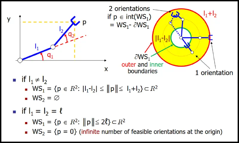
When dealing with inverse kinematics, an important notion are workspaces:

• primary workspace: set $\mathrm{WS}_1$ of positions $p$ that can be reached with at least one orientation
• secondary workspace: set $\mathrm{WS}_2$ of positions $p$ that can be reached with all orientations

Analytical solution (closed form)

• preferred (if it can be found)
• use geometric inspection, solve system of equations

Example: spherical wrist (3 revolute joins):

$$T_6^3(q) = \begin{bmatrix} c_4 c_5 c_6 - s_4 s_6 & -c_4 c_5 s_6 - s_4 c_6 & c_4 s_5 & c_4 s_5 d_6 \\ s_4 c_5 c_6 + c_4 s_6 & -s_4 c_5 s_6 + c_4 c_6 & s_4 s_5 & s_4 s_5 d_6 \\ -s_5 c_6 & s_5 s_6 & c_5 & c_5 d_6 \\ 0 & 0 & 0 & 1 \end{bmatrix}$$

The matrix $R$ is a ZYZ Euler rotation matrix and can be solved as such (see Body pose).

• we use indexes $3$ to $6$, because the wrist is usually at an end of another manipulator

For solving various manipulators (SCARA, for example), the law of cosines might also be quite useful: $$\begin{aligned} c^2 &= a^2 + b^2 - 2\ ab \cos \gamma \\ a^2 &= b^2 + c^2 - 2\ bc \cos \alpha \\ b^2 &= a^2 + c^2 - 2\ ac \cos \beta \end{aligned}$$

Definition (decoupling): dividing inverse kinematics problem for two simpler problems, inverse position kinematics and inverse orientation kinematics

• is applicable for manipulators with at least 6 joints where the last 3 intersect at a point
• the general approach is the following:
  1. calculate the orientations and position where the wrist needs to be
  2. calculate the orientations of the rest of the robot

Numerical solution (iterative form)

Two major ways of solving it, namely:

1. Newton method:
   • uses Taylor series around point $q_k$ to expand the forward kinematics $$r = F(q) = F(q_k) + \underbrace{\frac{\partial F(q_k)}{\partial q}}_{\text{Jacobian}\ J(q_k)}(q - q_k) + \underbrace{\mathcal{O}(||q-q_k||^2)}_{\text{neglected}}$$
   • stripping the higher-order terms and solving for $q$, we get $$\begin{aligned} r &= F(q_k) + J(q_k)(q - q_k) \\ r - F(q_k) &= J(q_k)(q - q_k) \\ J^{-1}(q_k)(r - F(q_k)) &= (q - q_k) \\ q = q_{k + 1} &= q_k + J^{-1}_r(q_k) \underbrace{(r - F(q_k)}_{\text{error}}) \end{aligned}$$
   • is nice when $n = m$, otherwise we have to use the pseudo-inverse
   • bad for problems near singularities (becomes unstable)
   • note: we’re using the Jacobian as a function here but it’s just a matrix
2. Gradient method:
   • aims to minimize the squared error (the $1/2$ is there for nicer calculations): $$H(q) = \frac{1}{2} ||F(q) - r|| = \frac{1}{2} [F(q) - r]^T [F(q) - r]$$
   • the gradient of $\nabla_q H(q)$ is the steepest direction to minimize this error: $$\nabla_q H(q) = J(q)^T [F(q) - r]$$
   • to move in this direction (given the current solution), we do the following: $$\begin{aligned} q_{k + 1} &= q_k - \alpha \nabla_q H(q_k) \\ &= q_k - \alpha J(q)^T [F(q) - r] \end{aligned}$$
     • $\alpha$ should be chosen appropriately (dictates the size of iteration steps)
   • we don’t use the inverse but the transpose, which is nice!
   • may not converge but never diverges

The methods could also be combined – gradient first (slow but steady), then Newton.

Velocity Kinematics

• relate linear/angular velocities $\dot{p}$ of the end effector to those of the joints $\dot{q}$
• again determined by the Jacobian matrix $J$ [nice overview video]
  • can be obtained either geometrically or by time differentiation
  • depends on the current configuration of the robot (encodes this information)
  • always a $6 \times n$ matrix: $$\begin{pmatrix} v_{EE} \\ \omega_{EE} \end{pmatrix} = \dot{p} = J(q)\dot{q} = \begin{pmatrix} J_L(q) \\ J_A(q) \end{pmatrix} \dot{q}$$

Two main cases when calculating the geometric Jacobian are the following:

	Prismatic Joint $i$
$J_{L_i} (q)$	$z_{i - 1}$	changes linear velocity (next joint moves linearly)
$J_{A_i} (q)$	$0$	doesn’t change the angular velocity
	Angular Joint $i$
$J_{L_i} (q)$	$z_{i - 1} \times p_{i - 1, EE}$	changes linear velocity too – moves next link $p$ is the vector from $i - 1$ to $EE$
$J_{A_i} (q)$	$z_{i - 1}$	changes angular velocity (next joint rotates linearly)

Where

• $z_{i - 1}$ is the orientation of the $z$ axis in the $(i - 1)$th frame and
• $p_{i-1, EE}$ is the distance from the center of the $(i - 1)$th frame to the end-effector
• $a \times b$ is the cross product between the vectors $a, b$, defined like this (just remember 2-3-1): $$a \times b = \begin{pmatrix} a_2 b_3 - a_3 b_2 \\ a_3 b_1 - a_1 b_3 \\ a_1 b_2 - a_2 b_1 \end{pmatrix}$$

And they can be calculated from the forward kinematics matrix (namely the DH matrices $A$): $$\begin{aligned} z_{i - 1} &= (\overbrace{R^0_1(q_1, \ldots, q_n)}^{\text{rotation part} \atop {\text{of matrix}\ A^0_1} } \cdot \ldots \cdot \overbrace{R^{i-2}_{i-1}(q_1, \ldots, q_n)}^{\text{rotation part} \atop {\text{of matrix}\ A^{i-2}_{i-1}} }) \overbrace{(0, 0, 1)^T}^{\text{just get\ }z} \\ p_{i - 1, EE} &= \underbrace{p_{0,EE} (q_1, \ldots, q_n)}_{\text{in last column of} \atop {\text{matrix}\ A^0_{EE} } } - \underbrace{p_{0, i - 1}(q_1, \ldots, q_{i - 1}}_{\text{in last column of} \atop {\text{matrix}\ A^{i - 1}_{EE} } }) \end{aligned}$$

Example: planar 2D arm:

	$a_i$	$d_i$	$\alpha_i$	$\vartheta_i$
1	$a_1$	$0$	$0$	$\vartheta_1^* = q_1$
2	$a_2$	$0$	$0$	$\vartheta_2^* = q_2$

$$J = \begin{pmatrix} z_0 \times p_{0,EE} & z_1 \times p_{1, EE} \\ z_0 & z_1 \end{pmatrix}$$

We now calculate $z$s and $p$s from the DH matrices:

$$A^0_1 = \begin{pmatrix} c_1 & -s_1 & 0 & a_1 c_1 \\ s_1 & c_1 & 0 & a_1 s_1 \\ 0 & 0 & 1 & 0 \\ 0 & 0 & 0 & 1 \end{pmatrix} \quad A^0_2 = \begin{pmatrix} c_{12} & -s_{12}& 0 & a_1 c_1 + a_2 c_{12} \\ s_{12} & c_{12} & 0 & a_1 s_1 + a_2 s_{12} \\ 0 & 0 & 1 & 0 \\ 0 & 0 & 0 & 1 \end{pmatrix}$$

We therefore get $$p_{0,1} = (a_1 c_1, a_1 s_1, 0)^T \qquad p_{0, EE} = (a_1 c_1 + a_2 c_{12}, a_1 s_1 + a_2 s_{12}, 0)^T$$

Since $p_{1,EE} = p_{0,EE} - p_{0,1}$, we get the $p$s and, as we see, $z_0 = z_1 = z_2 = (0, 0, 1)^T$

The full Jacobian matrix looks like this: $$J = \begin{pmatrix} z_0 \times p_{0,EE} & z_1 \times p_{1, EE} \\ z_0 & z_1 \end{pmatrix} = \begin{pmatrix} -a_1 s_1 - a_2 s_{12} & -a_2 s_{12} \\ a_1 c_1 + a_2 c_{12} & a_2 c_{12} \\ 0 & 0 \\ 0 & 0 \\ 0 & 0 \\ 1 & 1\end{pmatrix}$$

The rank of the matrix is between $1$ and $2$, depending on the joint configuration.

Higher-orders

For calculating other differential relations, we can just continue to derivate:

Relation	Equation
velocity	$\dot{r} = J_r(q) \dot{q}$
acceleration	$\ddot{r} = J_r(q) \ddot{q} + \dot{J_r}(q) \dot{q}$
jerk	$\overset{\ldots}{r} = J_r(q) \overset{\ldots}{q} + \dot{J_r}(q) \ddot{q} + \ddot{J_r}(q) \dot{q}$
snap	$\ldots$

Inverse Velocity Kinematics

• inverse problem to velocity kinematics
• for square non-singular $J$, we can just do $\dot{q} = J^{-1} (q) \dot{p}$
• has problems:
  • $\dot{q}$ is large near singularities
  • for redundant robots, we don’t have an inverse (see pseudo-inverse)

Singularities

In configurations where the Jacobian loses rank, we’re in a kinematic singularity – we cannot find a joint velocity that realizes the desired end-effector velocity in an arbitrary direction of the task space. Close to the singularity, the joint velocities might be very large and exceed the limits.

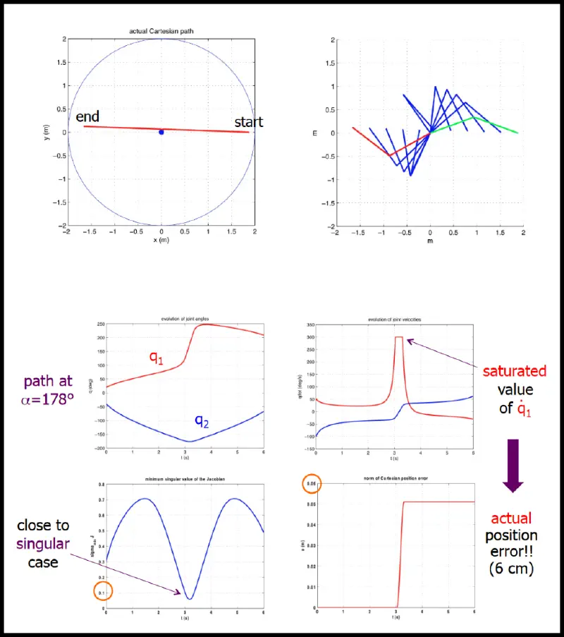
To remedy this, certain methods exist that balance error and velocity to make the robot movement smoother, like damped least squares, which minimizes the sum of minimum error norm on achieved end-effector velocity and minimum norm of joint velocity.

Pseudo-inverse

In the case that there is no solution to $J\dot{q} = \dot{p}$ (singularities, the robot simply can’t move that way, etc.), we still want to find a vector $\dot{q}$ that minimizes $$|| J \dot{q} - \dot{p} ||$$

This turns out to be the vector $\dot{q} = J^\# \dot{p}$, where $J^\#$ is the pseudo-inverse:

• can be obtained using SVD and
• satisfies the following conditions:
  1. $J J^\# J = J$
  2. $J^\# J J^\# = J^\#$
  3. $(J^\# J)^T = J^\# J$
  4. $(J J^\#)^T = J J^\#$

Force Kinematics

We can again use the Jacobian to relate forces of the end effector to those of the joints.

Given $\tau \in \mathbb{R}^{n \times 1}$ as the vector of infinitesimal joint forces/torques and $\gamma \in \mathbb{R}^{m \times 1}$ as the vector of infinitesimal end effector forces/torques. Applying the principle of virtual work (the work of the forces applied to the system are zero: ($dW = dF\ dx = 0$)), we get $$\begin{aligned} dW_\tau &= \tau^T\ dq \qquad & \text{\# joints} \\ dW_\gamma &= \gamma^T_e J(q)\ dq \qquad & \text{\# EE} \\ \forall \delta q \quad \delta W_\tau &= \delta W_\gamma \qquad & \text{\# virtual work} \end{aligned}$$

Simplifying, we get $$\tau = J^T(q) \gamma$$

This creates kinetostatic duality of the Jacobian

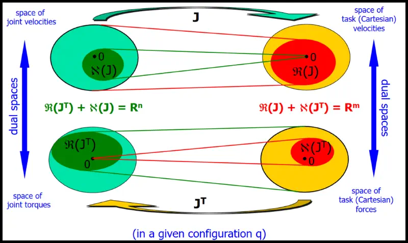
As a linear algebra reminder:

• $\mathrm{rank}(J)$: max number of rows/columns of $J$ that are linearly independent
  • $\mathrm{rank(J)} \le \min(m, n)$
  • if the rank of $J$ is full (typically $m$), then the robot’s EE can move in any direction; if not, there exists a direction in which the robot cannot move
• $\mathrm{range}(J)$: vector subspace generated by all possible linear combinations of columns of $J$
  • i.e. is a set of all possible values of where $J$ can map vectors
  • determines the velocities that EE can reach based on velocities of joints
• $\mathrm{kernel}(J)$: vector subspace generated by all vectors $v$ such that $Jv = \mathbf{0}$
  • i.e. is a set of all possible values of where $J$ maps to the vector $\mathbf{0}$
  • is the set of joint velocities that produce no EE velocity

Note that the problems are switched: compare the two equations $$\overbrace{\dot{p} = J(q)\dot{q}}^{\text{velocity kinematics}} \qquad \overbrace{\tau = J^T(q) \gamma}^{\text{(inverse) force kinematics}}$$

• for velocities, it is trivial to calculate the end-effector velocity from joint velocities
• for torques, it is trivial to calculate the joint torques from the end-effector torques

For completeness, here are some properties of the Jacobian and its transpose: $$\begin{aligned} \mathrm{range}(J) &= \left\{\dot{p} \in \mathbb{R}^m \mid \exists \dot{q} \in \mathbb{R}^n, J \dot{q} = \dot{p}\right\} \\ \mathrm{range}(J^T) &= \left\{\tau \in \mathbb{R}^n \mid \exists \gamma \in \mathbb{R}^m, \tau = J^T \gamma \right\} \\[0.5em] \mathrm{kernel}(J) &= \left\{\dot{q} \in \mathbb{R}^n \mid J \dot{q} = \mathbf{0}\right\} \\ \mathrm{kernel}(J^T) &= \left\{\gamma \in \mathbb{R}^m \mid J^T \gamma = \mathbf{0}\right\} \\[0.5em] \mathrm{range}(J) + \mathrm{kernel}(J^T) &= \mathbb{R}^m \\ \mathrm{range}(J^T) + \mathrm{kernel}(J) &= \mathbb{R}^n \end{aligned}$$

Trajectory Planning

Task: generate reference inputs to the controller when given:

1. only start and end defined (minimum requirements)
2. sequence of points defined (more difficult)

Definition (path): set of points in the joint space which the manipulator has to follow in the execution of the assigned motion (purely geometric).

Definition (trajectory): a path on which a timing is specified (velocities, accelerations, etc.).

• i.e. trajectory = geometric path + time law
• notation is $q = q(\lambda) \rightarrow \lambda = \lambda(t)$

To plan the trajectory, we do the following:

1. get the sequence of pose points (i.e. knots) in the Cartesian space
2. create a geometric path linking the knots (interpolation)
3. sample the path and transform the sequence to the Joint space
4. interpolate in the Joint space

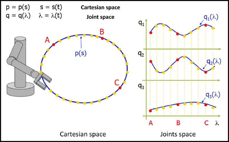
We do this because planning in the Cartesian space can easily move the robot into configurations that can’t be realized, which isn’t the case for the Joint space.

The time law is chosen based on task specification:

• stop at a point, move at constant velocity
• considers constraints and capabilities (max velocity, accelerations)
• may attempt to optimize some metric (min transfer time, min energy, etc.)

In Joint Space

Task: smoothly interpolate between points in the joint space

Cubic polynomial

Useful for interpolating between two positions ($q_0, q_1$) given the start and end velocity ($v_0, v_1$): $$q(0) = q_0 \quad q(1) = q_1 \quad q'(0) = v_0 \quad q'(1) = v_1$$

The cubic polynomial in the normalized form is the following: $$q(\lambda) = q_0 + \nabla q[a \lambda^3 + b \lambda^2 + c \lambda + d] \qquad \text{for}\ \nabla q = q_1 - q_0; \lambda \in \left[0, 1\right]$$

Plugging for known values helps us solve the polynomial:

• $q(0) = q_0 \Rightarrow d = 0$
• $q'(0) = \nabla q \cdot c \Rightarrow c = v_0 / \nabla q$
• $q(1) = q_1 \Rightarrow a + b + c = 1$
• $q'(1) = \nabla q \cdot (3a + 2b + c) \Rightarrow 3a + 2b + c = v_1 / \nabla q$

If we don’t care about normalization, the general form is the following: $$q(\lambda) = a \lambda^3 + b \lambda^2 + c \lambda + d$$

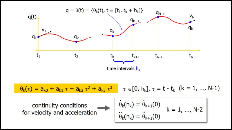
Splines

When we have $N$ knots and want continuity up to the second derivative, we can concatenate $N - 1$ cubic polynomials, which minimizes the curvature among all interpolating functions (with $2$nd derivatives)

• $4(N - 1)$ coefficients
• $4(N - 1) - 2$ conditions:
  • $2(N - 1)$ for the positions of the knots
  • $2(N - 2)$ for the continuity for first and second derivative at the internal knots
  • $\Rightarrow$ we have $2$ free parameters for assigning $v_1, v_N$

In Cartesian Space

Notation here is $p = p(s) \rightarrow s = s(t)$ (as opposed to $q = q(\lambda) \rightarrow \lambda = \lambda(t)$), since we’re planning the position of the end-effector, not the position in the joint space.

Has advantages and disadvantages:

• [+] allows more direct visualization of the generated path
• [+] can account for obstacles + lack of “wandering”
• [-] needs on-line kinematic inversion

When calculating the path:

• for simplicity, position and orientation are considered separately
• the number of knots is typically low (2 or 3), simple interpolating paths are considered

Position

Given $p_i, p_f, v_{\mathrm{max}}, a_{\mathrm{max}}$ and $v_{\mathrm{i}}, v_{\mathrm{f}}$ (usually $0$), we want to analyze the trajectory.

For a linear path from $p_i$ to $p_f$:

• path parametrization is $p(s) = p_i + s(p_f - p_i)$ with $s \in \left[0, 1\right]$
  • setting $s = \sigma / L, \sigma \in \left[0, L\right]$ (given the length of the path)
• we can differentiate to get velocity and acceleration: $$\begin{aligned} \dot{p} &= \frac{dp}{ds}\dot{s} &= (p_f - p_i) \dot{s} = \frac{p_f - p_i}{L} \dot{\sigma} \\ \ddot{p} &= \frac{d^2s}{ds^2} \dot{s}^2 + \frac{dp}{ds}\ddot{s} &= (p_f - p_i) \ddot{s} = \frac{p_f - p_i}{L} \ddot{\sigma} \\ \end{aligned}$$

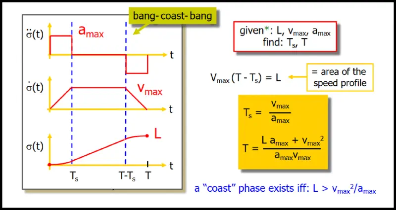
For the motion, we use the trapezoidal speed (bang-coast-bang):

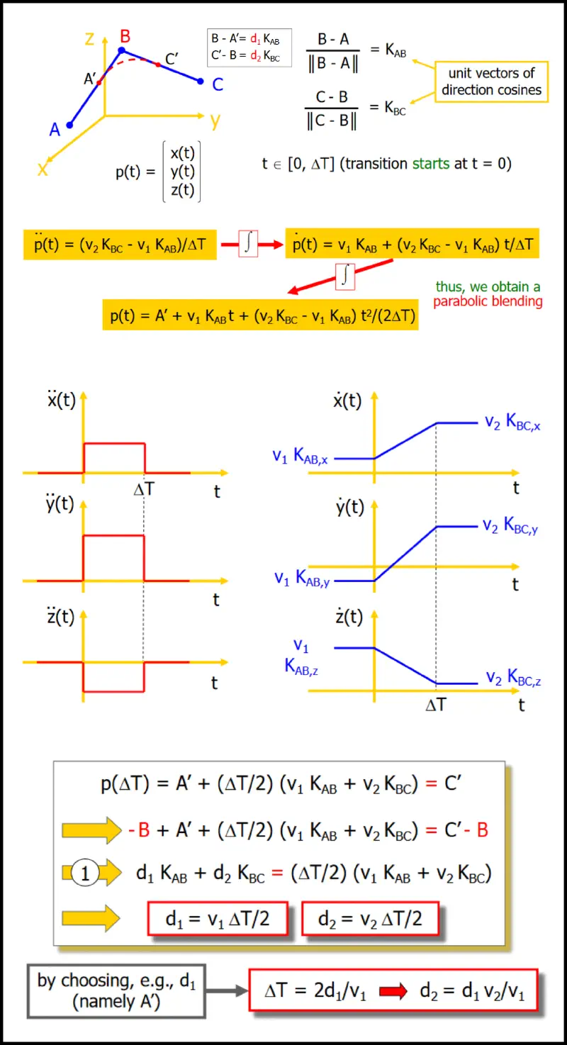
To generalize this (i.e. concatenate the paths), we can over-fly the point in between. A specific example of how this would look like is the following:

Orientation

1. use minimal representations (e.g. ZYZ Euler angles) and plan the trajectory independently
2. use axis/angle representation:
   • determine a neutral axis and an angle by which to rotate
   • plan a timing law to interpolate the angle and the axis

Optimal trajectories

For Cartesian robots (PPP):

1. straight line joining the two positions is one of those
   • can be executed in minimum time under velocity-acceleration constraints
2. optimal timing law is the bang-coast-bang

For articulated robots (at least one R):

• 1. and 2. are no longer true in general case, but time-optimality still holds in the joint space
     • note that straight lines in joint space don’t correspond to those in Cartesian space!

Uniform time scaling

Say we want to slow a given timing law down or speed it up because of constraints, we don’t need to recalculate all of the motion profiles: velocity scales linearly, acceleration scales quadratically: $$\begin{aligned} dp/dt &= dp/ds \cdot ds/d\tau \cdot {\color{red}{1/T}} \\ d^2p/dt^2 &= (d^2p/ds^2 \cdot (ds/d\tau)^2 + dp/ds \cdot d^2s/d\tau^2) \cdot {\color{red}{1/T^2}} \end{aligned}$$

Example (max relative violations) with $T = 1 [\mathrm{s}]$:

• $k_{\text{vel}} = \max \left\{1, |\dot{q}_1| / v_{\max,1}, |\dot{q}_2| / v_{\max,2}\right\}$
• $k_{\text{acc}} = \max \left\{1, |\ddot{q}_1| / a_{\max,1}, |\ddot{q}_2| / a_{\max,2}\right\}$

Minimum uniform time scaling is therefore $$k = \max \left\{1, k_{\text{vel}}, \sqrt{k_{\text{acc}}}\right\}$$

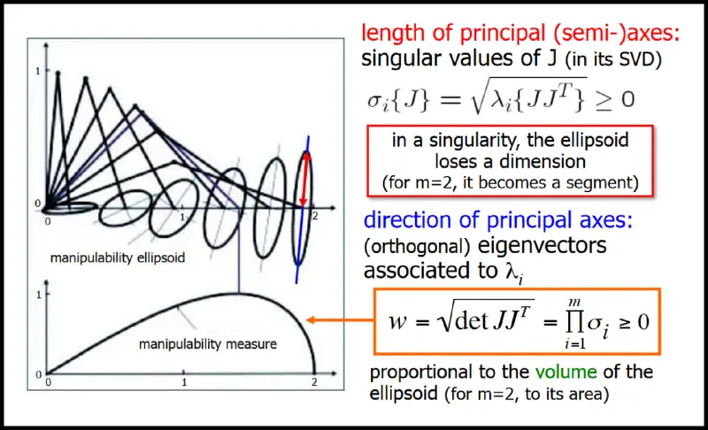
Manipulability

Velocity manipulability

In a given configuration, we want to evaluate how „effective“ is the mechanical transformation between joint velocities and EE velocities (how „easily“ can EE move in various directions of the task space).

• we consider all EE velocities that can be obtained by choosing joint velocities of unit norm:

$$\dot{q}^T \dot{q} = \underbrace{v^T J^{\#T}J^\#v}_{\text{ellipsoid}} = 1$$

Force manipulability

We can apply the exact same concept to forces:

$$\tau^T \tau = \underbrace{F^TJJ^{T}F}_{\text{ellipsoid}} = 1$$

The comparison between the two is interesting – they are orthogonal (velocity left; force right):

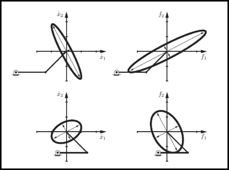
The explanation that the teacher gave in class is pretty good: if your arm is almost stretched, it can move very quickly up and down but not too quickly forward/backward. On the other hand (pun not intended), the forces you can apply up/down are not nearly as large as when pushing/pulling.